


It is impossible to have an intelligent discussion of economics, of game theory, or of behavioral economics – let alone their successes and failures – without some idea of what they are about. Homo economicus is a far different creature than commonly imagined. Let us begin by examining this mythical construct more closely.
What is Game Theory?
The heart of modern “rational” economic theory is the concept of a non-cooperative or “Nash” equilibrium of a game. If you saw the movie A Beautiful Mind this theory – created by Nobel Laureate John Nash – is briefly described, albeit inaccurately. But to put the oxen before the cart, let us first describe what a game is. A game in the parlance of a game theorist or economist does not generally refer to a parlor game such as checkers or bridge, nor indeed to Super-Mario III. Instead, what economists call game theory psychologists more accurately call the theory of social situations. There are two branches of game theory, but the one most widely used in economics is the theory of non-cooperative games – I shall describe that theory here.
The central topic of non-cooperative game theory is the question of how people interact. A game in the formal sense used by economists is merely a careful description of a social situation specifying the options available to the “players,” how choices among those options result in “outcomes,” and how the participants “feel” about those outcomes. The timing of decisions and the information available to players when undertaking those decisions must also be described.
The critical element in analyzing what happens in a game (or social situation) is the beliefs of the players: what do they think is likely to happen? How do they think other players are likely to play? From a formalistic perspective the beliefs of players are generally described by probability distributions – we assign a probability to an outcome – although in more advanced theories – such as epistemic game theory – beliefs are more sophisticated and mathematically complicated objects. Please observe that the notion that we are uncertain about the world we live in and about the people we interact with is at the very core of game theory.
Given beliefs about consequences and sentiments about those outcomes it is almost tautological to postulate that players choose the most favorable course of action given their beliefs. At one level this is what it means for players to be “rational” and should scarcely be controversial… yet many dense books have been written criticizing this notion of rationality.
Of course a theory that says that players believe something and do the best they can based on those beliefs is an empty theory because it does not say where beliefs come from. I sell my stocks? I must believe the market is going down. I spend all my money? I must believe the world is coming to an end. And so forth. The formation of beliefs is at the center of modern economic theory.
Our beliefs surely depend on what we know. I believe that if I drop this computer it will fall to the ground – because I have a lifetime of experience with falling objects. By way of contrast I have no idea when I wake up tomorrow morning whether the stock market will have gone up or down, and even less what might be the consequences of clean coal technology for global warming over the next decade.
Historically the economics profession has been most interested in situations where the players are experienced. For example, investment decisions are typically made by investors with long and deep experience of investment opportunities; most transactions are concluded between buyers and sellers with much experience in buying and selling. Under these circumstances it is natural to imagine that beliefs reflect underlying realities. In the theory of competitive markets this has been called rational expectations. In game theory it is called Nash equilibrium. Notice, however, that such a theory does not demand that people know the future – we call that “perfect foresight” not “rational expectations” – only that the probabilities they assign to the future are the same probabilities shared by other equally experienced individuals. Put differently: while I have no idea whether when I wake up tomorrow morning the stock market will have gone up or down, I do know that both outcomes are about equally likely. As this view is widely shared, it represents “rational expectations” about tomorrow’s stock prices.
Another way to describe Nash equilibrium is this: Nash equilibrium represents a setting in which no further learning is possible. That is – if some player holds wrong beliefs the possibility exists that they will discover their mistake and learn something new. When possibilities for learning are exhausted what we find is Nash equilibrium.
How well does the theory of Nash equilibrium work? One of the most widely used empirical tools in modern behavioral economics is the laboratory experiment in which paid participants – many times college undergraduates, but often other groups from diverse ethnic and social backgrounds – are brought together to interact in artificially created social situations to study how they reach decisions individually or in groups. Many anomalies with theory have been discovered in the laboratory – and rightfully these are given emphasis among practitioners – we are, after all more interested in strengthening the weaknesses in our theories than in simply repeating that they are correct. Amidst all this the basic fact should not be lost that standard economic theory works remarkably well in the laboratory.
Let me be more specific. Let us take as our theory the theory of Nash equilibrium. Let us also suppose (we will talk more about this later) that laboratory subjects care only about bringing home the most possible money from the experiment. Do we observe Nash equilibrium in the laboratory?
Voting
One of the most controversial applications of the theory of rational man is to voting. Modern voting theory, for example the 1996 theory of Feddersen and Pesendorfer, is based on the idea that your vote only matters when it decides an election – when your vote is pivotal. This has implications for voter participation. If elections are not close there is no chance of your vote mattering, and no incentive to participate. To be an equilibrium, elections must be so close that the chance of changing the outcome is enough to compensate for the cost of participating. Whether this is how voters behave is quite controversial: it is often referred to as “the paradox of voter turnout.” It is central to Green and Shapiro’s harsh 1994 critique of rational choice theory in which they assert that
Those tests that have been undertaken [of rational choice theory] have either failed on their own terms or garnered theoretical support for propositions that, on reflection, can only be characterized as banal: they do little more than restate existing knowledge in rational choice terminology.
In 2007 Levine and Palfrey examined voter participation in the laboratory. Our subjects were UCLA (University of California, Los Angeles) undergraduates. After arrival at the laboratory the subjects were divided into unequal teams of voters. Later, various elections were conducted: in some elections one “party” had a 2/3rds majority, in others a one-vote majority. We conducted elections with numbers of participants ranging from three to fifty-one.
In these elections voters had a choice between casting a vote for their own party and abstaining. Voters received a small payment for participating in the experiment plus the members of each winning party received a prize of $0.37 each. This was split between the two parties in case of a tie. Voting in the laboratory – as in real life – was costly. Each voter was randomly assigned a cost of voting ranging from $0.00 to $0.185. This cost was known only to the voter to whom it was assigned – all other aspects of the experiment were commonly known to all the voters.
Notice that in this setup the most you can hope to do is to swing a losing election to a tie, or swing a tie to a win, in either case garnering an additional $0.185. So if you drew the lowest voting cost of $0.00 it makes sense to vote as long as there is even a small chance of changing the outcome, while if you drew the highest cost of $0.185 you would never vote unless you were absolutely certain to change the outcome. For other costs whether it is a good idea to participate or not depends on how likely you think you are to alter the outcome. For instance, if you think the probability of influencing the election is high you should accept a higher cost of voting.
Sticking with the (not entirely plausible) assumption that voters are strict moneygrubbers, it is possible but not easy to compute the Nash equilibrium of this game. Depending on the probability of making a difference there is a threshold cost below which it is rational to vote, and above which it is not – this is known as a “cut-off” decision. The participation rate is determined by this threshold – the higher the threshold, the higher the participation rate. Conversely the higher the participation rate, the less likely it is that voters make a difference. This kind of interdependence is described by economists and mathematicians as a fixed-point problem, and requires solving – in this case – some rather complex non-linear equations. This can be done only on the computer, and while in principle there could be more than one solution to these equations, in fact there is only one. Thus using the computer we made this difficult calculation determining for each election what was the Nash equilibrium.
As indicated, we then re-created the theoretical environment in the laboratory. We had no expectation that voters could guess, calculate, or otherwise intuitively figure out how best to behave – as I mentioned it is quite a complex problem. Rather, as is central to modern economic theory (see the quote of Lucas above), we imagined that if voters were given an opportunity to learn they would reach an equilibrium. Hence, we gave them ample opportunity to learn – voters got to participate in fifty elections each.
To measure how well the theory worked we focused on how likely it was for a player to make a difference. A pivotal event in this experiment is a situation that is either a tie, or one party wins by a single vote. Since voters only participate because they have a chance of being pivotal, in equilibrium the chance of such an event cannot be too small. Since elections “often” have to be close, it follows that there must also be upsets in which the minority party wins. The theory also predicts how frequently this will occur. For each type of election we computed what was the probability of pivotal events and upsets. For those of you familiar with social science research, you should notice what we did not do. We did not collect a bunch of data about behavior and fit a curve to it and declare that our curve “fits the data well” or is “statistically significant.” We did not declare that if there are more voters the participation rate should be “lower.” For any election with any number of voters, and any size of prizes and probabilities of drawing participation costs the theory of Nash equilibrium makes precise quantitative predictions about the frequency with which we should observe elections results that are pivotal and elections that result in an upset.
What happened with real people in our experimental laboratory? The figure below shows the results on a graph in which the horizontal axis has the frequencies we computed from the theory of Nash equilibrium and the vertical axis has the corresponding frequencies of actual election results in the laboratory. Each different election setting with different numbers of voters in each party corresponds to a different point on the graph. If the theory worked perfectly all of these points should lie on the 45 degree line where the theory exactly matches the data – for instance if the theory predicts 0.4 then we should observe 0.4. As you can clearly see – that is exactly what happens – the theory works more or less perfectly. If you do not believe this, try dropping tennis balls out your window and calculating the force of gravity and see how accurate your measurement is. Less good than this I can assure you.
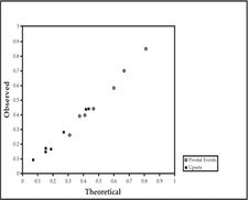
Probability of Pivotal and Upset Elections
Let us again emphasize what we did not do. Often when social scientists say their theory fits the data what they mean is that they “estimated free parameters” and given their best estimate of those parameters the corresponding model reflects the data. This would be as if instead of saying that our observations should lie on the 45 degree line, we said they should lie on some unknown line – the slope and intercept of that line being “free parameters” – and declaring victory if we could find a line that more or less passed through the data. Here there are no free parameters; nothing is estimated, there are no unknowns. We take the information about the setting – how many voters; what prizes, and so forth – and we calculate a number – the probability of a pivotal event or upset using the sharp predictions of Nash equilibrium. This number is then either right or wrong – in fact it is right. But there is no wiggle room to “estimate parameters” or otherwise fudge around with things.
Economics is a Quantitative Subject
The voting experiment illustrates what economics is and what it is not. It is not about the intersection of supply and demand curves, and about what direction prices move if a curve “shifts.” It is a quantitative theory of human behavior both individually and in interaction with other people.
The importance of the quantitative nature of economics often eludes clever observers, especially philosophers and lawyers. Take for example the following (possibly apocryphal) quotation – from the “original” behavioral economist Kenneth Boulding
anyone who believes exponential growth can go on forever in a finite world is either a madman or an economist.
This appears to involve a straw man, since as far as I know no economist would argue that exponential growth can go on forever – at best this is something we are uncertain about. The point is not debatable. But what conclusion can we draw from the fact that exponential growth cannot go on forever? Boulding evidently would like us to conclude that if it cannot go on forever, it cannot go on for very long. Of course that does not follow. Exponential growth might be possible for only the next ten years – or it might be possible for the next ten thousand years. If the latter, there is hardly any point in arguing over it – and a model in which exponential growth can go on forever can certainly be useful and relevant despite its obvious falsity. On the other hand if we are going to run out of resources in ten years time – then indeed fooling around with models of exponential growth is a waste of time.
The point is that philosophers’ and lawyers’ reasoning – trying to draw a practical conclusion from an extreme hypothetical statement – “exponential growth cannot go on forever” – is false reasoning. All the action is in the quantitative dimension: some numbers are big, some numbers are small and how big and how small matters, not whether numbers are exactly equal to zero, or “infinite.”
Here is a practical application of quantitative reasoning: let’s consider whether or not torture should be against the law. Notice the question is not whether or not torture is “good” or “bad” or whether it is “moral” or “immoral.” A standard argument that torture should be legal is based on a simple hypothetical choice experiment. Many people if faced with a choice of torturing a suspect to determine the location of a nuclear weapon set imminently to explode in a large city would be in favor of doing so. Under those circumstances I would be prepared to do so. The conclusion is then derived that torture should be legal under these circumstances, and therefore the debate should be about when not whether torture should be legal. But in fact the conclusion does not follow.
As I indicated I would be willing to torture a suspect under the specified circumstances – yet I believe that it should be illegal for me to do so. Of course were I to be brought to trial I would hope to be let off on the grounds of necessity, or to get a Presidential pardon – but the point is that because the act is illegal – hopefully with severe penalties – I would certainly not be inclined to torture someone for frivolous reasons. Thus here is an economic argument against legalizing torture: if it is legal, despite the limited the circumstances under which it is legal, then – in practice – there will be far too much torture. By the way – the evidence is overwhelming – in every instance in which a government has bureaucratized torture it has quickly gotten out of hand. But again the basic point: from an economic point of view the issue is not “will there be torture” or “will there not be torture” but “what will be the impact of making torture legal or illegal on the amount of torture that is practiced.” Hypotheticals about nuclear bombs in cities do not help us answer this quantitative question.
I should also add a warning at this point. Be careful in debating lawyers and philosophers. At this point in the argument they will introduce yet another irrelevant hypothetical “suppose that torture can be made legal without leading to excessive torture – should it be legal then?” To which the only relevant answer is “don’t waste my time.”
If – as is likely – you aren’t planning on debating any lawyers or philosophers over economic issues – at least when a behavioral economist insists that people exhibit this or that form of irrationality, please ask: how many people and how irrational is the behavior in question? Theories by their nature are false. The question is always – are they quantitatively useful or not?
The Rush Hour Traffic Game
Beware of lawyers and philosophers bearing hypothetical examples. But beware also of social scientist bearing only laboratory results. After all – our main interest is: does the theory work outside the laboratory? In particular – does Nash equilibrium work outside the laboratory? That question is easier to answer than you might think.
There is a game that most of us are intimately familiar with. It is played five days a week in every major city in the world: it is the rush hour traffic game. In the “morning game” the “players” are commuters trying to get to work. Their choices are which route to take. Their objective is to minimize the time it takes to get to work – the more time it takes to get to work, the less happy you are. A moment of reflection should convince you that the sheer size of this game is overwhelming – in a large city it involves millions of players each of whom chooses between millions of routes. Yet the outcome of this game is a Nash equilibrium.
Wow! How can I possibly know that? Even the biggest supercomputer in the world can’t compute the Nash equilibrium of this game. Recall, though, what a Nash equilibrium is. It simply means that each commuter is taking the quickest route given the routes of all the other commuters. So the test of the Nash equilibrium theory is a simple one: are there commuters who can find quicker routes?
This test, by the way, is why I want to focus on rush hour traffic. During non-rush times there are many inexperienced drivers on the road, some making one of a kind trips to unfamiliar locations, and often they take routes that are much slower than the fastest available. Nonetheless during rush hour commuters are experienced, and have tried a lot of routes in the past – there is no much room for learning. So – if you try to take a tricky combination of side streets rather than the main boulevard you discover that just enough traffic has spilled over on to the side streets that you can gain no advantage. How do I know this? I’ve tried – I suggest you do. For years I commuted about an hour to work through Los Angeles rush hour. I was often stuck on a very slow boulevard in Beverly Hills. In frustration I experimented with many alternative combinations of side streets. Sadly it never got me to work faster. In fact on one occasion, I was behind a large truck when I got off the main boulevard, and after ten minutes of tricky driving, I got back on the main boulevard – just to find myself behind exactly the same truck. In short: Nash equilibrium.
Now you may believe that I am right that what we observe at rush hour throughout the world is a Nash equilibrium. You may also wonder – since we can’t possibly compute what it is – what good that observation does us. As it transpires it does us quite a bit of good – but we’ll talk about that in the next chapter.
Economists who study voting and traffic patterns are few and far between. For the most part what economists study is trade taking place in markets. And few things seem more controversial than the assertion that markets “clear.” Or that markets are competitive when there are only a handful of firms. For example a former Presidential advisor, N. Gregory Mankiw writes
New Keynesian economists, however, believe that market-clearing models cannot explain short-run economic fluctuations. (2010)
Given this controversy, the experimental evidence may surprise you: it is easy to identify what settings are competitive, and in these settings we observe exactly the price that economists expect based on theory.
The most striking example is the work by Roth et al. in 1991 examining a simple market auction with nine identical buyers. These buyers must bid on an object worth nothing to the seller, and worth $10.00 to each of them. If the seller accepts he earns the highest price offered, and a buyer selected from the winning bids by lottery earns the difference between the object’s value and the bid. Each player participates in 10 different market rounds with a changing population of buyers. In all these possible situations, bids must be in increments of five cents.
What does game theory predict should happen? Suppose the highest bid is some amount, call it in the time honored tradition, x. If you bid x then there is a tie and you have at most a 50% chance of getting the object and can earn at most an expected payoff of ($10 – x)/2. If you raise the bid by a nickel – you get the object with certainty – you can earn $ 9.95 – x. As it happens if x < $ 9.90 it is better to raise by a nickel and get $ 9.95 – x rather than ($10 – x)/2. Also if x < $10 you never want to bid less than x since then you would get nothing, while by bidding x you would get a share of something. Finally, if everyone else bids $9.90 you can do better by bidding $9.95 getting the entire five cents for yourself, rather than a 1/9th share of ten cents. Therefore at a Nash equilibrium the winning bid has to be at least $9.95 and of course it cannot be more than $10.00.
So what happened in the laboratory? By the time the participants had played in seven auctions the price was $9.95 or $10.00 in every case – and in most cases this happened long before the seventh try.
Notice the key feature of this auction: no individual buyer can have much impact on the price: since everyone else is bidding $9.95 or $10.00 the question for a buyer is not so much about changing the price, but rather their willingness to buy given that price. This idea – that market participants can have little impact on prices – is a central one in the economic theory of competitive markets. The corresponding theory – the theory of competitive equilibrium – is an important variation on Nash equilibrium. It is a theory in which traders in markets choose their trades ignoring whatever small impact they may have on market prices. Equilibrium occurs at prices that reconcile the desire of suppliers to sell with consumers to buy.
At one time a great deal of effort was expended by economists trying to understand the mechanism by which prices adjusted. Modern economic theory recognizes that the particular way in which prices are adjusted is not so important. An important modern branch of game theory is mechanism design theory. While game theory takes the game as given, mechanism design theory asks – how might we design a game to achieve some desired social goal? To emphasize that the choice of the game is part of the problem, the way in which decisions of players are mapped into social outcomes is called a mechanism rather than a game.
From the mechanism design point of view, an auction is just one of many price setting mechanisms. It is a mechanism that acts to reconcile demand with supply – to clear the market. There are many mechanisms that do this. They are all equivalent in that they perform the same function of clearing markets. Consequently the exact details are of no great importance. Perhaps it is done electronically as it is the case with the Chicago Board of Trade. Or, perhaps, by shouting out orders as on the New York Stock Exchange (NYSE).
How well does the theory of competitive equilibrium and market clearing work? Let’s consider a simple market with five suppliers. Suppose that each supplier faces a cost of producing output given by the following table:
Units Produced |
Cost |
0 |
0 |
20 |
905 |
40 |
1900 |
60 |
3000 |
240 |
17000 |
Supplier Cost
The profit of a firm is just the amount it receives from sales – its revenue – minus this cost. For any particular price we can work out from the cost data how many units should be produced to maximize profits:
Price |
Profit Maximizing Output |
Corresponding Industry Output |
100 |
240 |
1200 |
90 |
198 |
990 |
60 |
72 |
360 |
30 |
0 |
0 |
10 |
0 |
0 |
Profit Maximizing Output
I did this computation using calculus – and that is why we demand our undergraduate students know calculus. But obviously business people do not generally choose their production plans by using calculus. Rather they weigh the cost of hiring a few more workers against the additional revenue from a few more sales and decide whether or not to expand – or shrink – their operation. Of course in the end they get exactly the same result as I do by using calculus.
The price that consumers will pay depends on how many units are offered for sale in total. Suppose that this is given by the demand schedule
Units for Sale |
Sale Price |
0 |
100 |
180 |
80 |
360 |
60 |
630 |
30 |
900 |
0 |
Demand Curve
Notice that for the firms to decide how much to produce they must guess what price they will face. In the competitive market clearing equilibrium – also called the rational expectations or perfect foresight equilibrium – they guess correctly. Inspecting the table for profit maximization – the supply, and the table for consumer willingness to pay – the demand, we see that when price is 60 consumers wish to purchase 360 units, and firms wish to provide this same number. Thus 60 is the price that “clears the market” or the “competitive equilibrium price.”
Bear in mind that in a competitive equilibrium firms are strategically naïve. They ignore the fact that by producing less there will be less supply and consumers will be willing to pay more resulting in a higher profit. Since each firm is only 20% of the market the ability of an individual firm to manipulate prices is not large, but it is not zero either. If we apply the theory of Nash equilibrium so that each firm correctly anticipates the choices of their rival firms, then firms produce less – 63 instead of 72 – and the Nash equilibrium price is higher: 65 rather than the competitive price of 60. The difference between the Nash and competitive equilibrium is not all that great, so that even with as few as five firms, competitive equilibrium with market clearing is a reasonable approximation.
Undoubtedly, real people are not unboundedly rational. They can scarcely be expected to rationally forecast “equilibrium” prices. Let us instead consider a “behavioral” model: let us suppose that firms forecast prices next period to be whatever prices were last period. This is exactly the behavioral model of adaptive expectations formation that was widely used before the rational expectations revolution of which behavioral economists are so critical.
What happens when prices are forecast to be the same next period as last? If the starting price is 90, then firms will wish to produce 990 units of output. Consumers are not willing to buy so many units, so price falls to 0. At that price firms aren’t willing to produce anything, so now price then rises to 100. The following period the industry produces 1200. The cycle then continues with the market alternating between overproduction leading to a zero price, then underproducing leading to a price of 100. This is the so-called “cobweb” although we might also refer to it as a business cycle – the failure of the capitalist system by flooding the market with cheap goods and then falling into recession. Karl Marx pointed out exactly this self-destructive tendency of capitalism.
Which theory is correct? In 2004 Sutan and Willinger implemented this market in the laboratory with real subjects playing for real money. Participants had an opportunity to play variations of this game 40 times. There were three different experimental markets. The graph below plots the actual price in each of those markets against the number of times players interact in those markets:
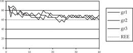
Market Prices over Time
After about the first ten periods prices fluctuate within a relatively narrow band in all three markets. It is generally higher than the rational expectations competitive price of 60, which is marked by the dotted line in the graph. Interestingly Sutan and Willinger view this as a minor contradiction of economic theory. In fact the subjects are cleverer here than the experimenters: the price is essentially the Nash equilibrium price of 65. As we shall see later it is not so uncommon for subjects to outwit experimenters. Often “anomalous” experimental results supposedly contradicting economic theory simply reflect the fact that the experimenter misunderstood what the theory says. As the fundamental theory is that of Nash equilibrium which predicts a price of 65 – the results of this experiment are just what the theory predicts. Competitive equilibrium is merely an approximation. Here it is a useful approximation as the competitive price of 60 is close to the Nash equilibrium price of 65, but it is not exact.
By way of contrast the behavioral theory does about as badly as a theory can. The average price according to the behavioral theory is 50 – much lower than the actual market price which is always above 60 – and prices remain within a tight band – they certainly do not cycle abruptly from 0 to 100.
The key point here is that while it is no doubt true that people do not have unbounded rationality, we have only very simple and naïve models of bounded rationality. It is a fact that people are very good at learning, and even very sophisticated computer programs produced over many years by very skilled computer scientists working on artificial intelligence are much less capable of learning than even small children. By contrast “behavioral” models of “bounded rationality” such as expecting next period price to equal this period price are extremely simplistic. Hence the quantitative question: is a model of unbounded rationality or an extremely primitive model of learning a better approximation to reality? In this experiment it is clear that the model of unbounded rationality is vastly better.
The results of this experiment are by no means atypical. Experiments on competitive equilibrium have been conducted many times, dating back at least to the work of Vernon Smith in 1962 – work that is hardly obscure as he won a Nobel Prize for it. Most of these experiments involve real paid subjects in the role of both buyer and seller. The results are highly robust: competitive equilibrium predicts the outcome of market experiments with a high degree of accuracy, with experimental markets converging quickly to approximately the competitive price.