


7. Behavioral Theories II: Time and Uncertainty
The previous chapter discussed various irrationalities and biases alleged by behavioral economists. Much of the work in behavioral economics, however, has focused on the elements of time and uncertainty. Unlike the biases of the previous chapter – which generally attack issues that are not of great interest to economists – time and uncertainty lie at the very heart of modern economics. So let us examine these topics from the behavioral point of view.
Present Bias
One distinguished critic of “standard economics” is David Laibson of Harvard who had drawn the profession’s attention to the phenomenon known as present bias. As an example, most people given a choice between $175 today and $192 in four weeks time will take the immediate payoff of $175. On the other hand given a choice of $174 in 26 weeks time and $192 in 30 weeks time (also four weeks later) most people will take the $192. The data from Keren and Roelofsma [1995] below puts specific numbers to this.1
Choices |
Fraction Making Choice |
|
1 |
$175 now |
0.82 |
$192 in 4 weeks |
0.18 |
|
2 |
$175 in 26 weeks |
0.37 |
$192 in 30 weeks |
0.63 |
Fraction of People Making Choice2
This type of behavior has been long established in psychology, for example, in the 1996 work of Green and Myerson. Notice that the fact that people discount the future is present in virtually all of economic thought. Yet present bias violates the standard economic model in which people discount the future using geometric weights.
The first thing to observe is that this type of present bias is only apparently inconsistent with the standard model of geometric discounting. A number of economists such as Fernandez-Villaverde and Mukherji [2003] have pointed out that in practice we have much more knowledge of our immediate desires than our future desires. That is: some of us could really use some money today rather than in four weeks time and we know it. Still, many fewer of us know that twenty-six weeks from now we will be in desperate need of a cash infusion. In the presence of uncertainty we may well observe what appears to be a “present bias” even with standard homo economicus.
Present bias raises yet another issue: if we really feel today that we’d rather have $192 in thirty weeks time than $175 in twenty six weeks time but, given the choice, twenty six weeks from now rather than today would choose the $175 then there is a conflict between our current self and our future self. So given a choice today between $175 in twenty six weeks, $192 in thirty weeks, or being allowed to wait and make the decision twenty six weeks from now – some of us would choose the $192 over the option of waiting. This can’t be due to uncertainty about our future desires: in that case the best thing to do is wait and see what they are. A single rational decision maker would always prefer the flexibility of waiting, so self-commitment – intentionally limiting our future options – is not consistent with standard economic models.
It is not so hard to think of examples of self-commitment. The Nobel Prize winning game theorist Tom Schelling tells a story of trying to stuff a carton of cigarettes down the garbage disposal in the middle of the night. Given the likely effect on the garbage disposal this cannot have been a good idea – but the reason for it was sound enough; he was afraid of facing the temptation of smoking and wanted to take it off the table. A less obvious example can be found in DellaVigna and Malmendier’s 2006 study of health club memberships. People who chose long-term memberships rather than pay per visit paid on average $17 per visit against a $10 per visit fee. Leaving aside the hassle factor of availability of lockers and the need to pay each visit, we can agree that this is some evidence that people are trying to make a commitment to attending the health club.
As we said, in the idealized world usually studied by economists, there is no need for a single decision-maker ever to commit. In reality we often choose to make commitments to avoid future behavior we expect to find tempting but with bad long-term consequences: the drug addict who locks himself in a rehab center would be another obvious example. The long-term membership in a health club has a similar flavor. Skipping a workout can be tempting but has bad long-term consequences for health. Having to pony up $10 makes it easier to find excuses to avoid going.
There is little new under the sun: the economist Richard Strotz was studying problems of self-commitment in the rather mainstream Review of Economic Studies back in 1955. However the type of models he proposed were not widely used until the “behavioral economics revolution.” Two models that have come into widespread use are called respectively hyperbolic and quasi-hyperbolic discounting (also known as the beta-delta model) – as opposed to the more ordinary and familiar geometric sort of discounting. David Laibson’s [1997] paper examining the consequences of hyperbolic discounting models for consumption behavior – a topic of great interest to economists, although quite possibly nobody else – was published in the also mainstream Quarterly Journal of Economics and has been cited some 1543 times, so cannot be said to have been overlooked. The only problem with the model is that it predicts that present bias should not depend on whether or not the reward is uncertain. Unfortunately this is not the case.
Choices |
Probability of reward3 |
||
Scenario |
1.0 (60) |
0.5 (100) |
|
1 |
$175 now |
0.82 |
0.39 |
$192 in 4 weeks |
0.18 |
0.61 |
|
2 |
$175 in 26 weeks |
0.37 |
0.33 |
$192 in 30 weeks |
0.63 |
0.67 |
|
Fraction Making Choice with Uncertain Reward
Turning back to the data from Keren and Roelofsma [1995] as displayed in the table above – they examined what happened to preference reversals when there was only a 50% chance of getting the money.
A fair summary of the data is that when the chance of reward is only 50% people behave pretty much the same way with respect to both the present and future reward as they do with a certain future reward. If a non-standard model of discounting is needed to understand the first column, the standard model is needed to understand the second. This makes it hard to argue that the “behavioral” model is better than the standard one.
While it isn’t at all obvious that present bias has much to say about why we have economic crises or some countries are so poor, the topic has still gained the interest of economists, even economists such as the Princetonian pair Faruk Gul and Wolfgang Pesendorfer who are strongly declared opponents of any notion of behavioral. In 2001 the two wrote a paper proposing that people have preferences over menus – lists of which options will be available – that exhibit a preference for commitment. Dekel, Lipman and Rustichini proposed a similar model at about the same time. Variants of these models including models of internal conflict called self-control models are a major topic of ongoing research. For example, the enormously distinguished and mainstream economists Drew Fudenberg and David Levine wrote about self-control models in the American Economic Review in 2006 and again in Econometrica in 2012.
Models of self-control may reasonably be described as behavioral: they postulate that rather than a single decision maker each of us has several conflicting selves and that the resolution of internal conflict leads to our final decisions. These models were pioneered by behaviorists: Shefrin and Thaler in 1981 and Ainslie in 2001. They have an obvious role in explaining things such as impulsive behavior and drug addiction. On the other hand, while I personally think that these types of models have a great deal to say about behavior – there is still a need for caution in interpreting what people do.
The fact is that a lot of behavior that is commonly thought to be impulsive – spur of the moment, giving in to temptation and taking immediate gratification at the expense of the future – is nothing of the sort. Gambling and sexual behavior are common examples of supposedly impulsive behavior. Nevertheless this so called “impulsive” behavior – giving in to temptation – is often anything but. Take Eliot Spitzer who lost his job as governor of New York because of his “impulsive” behavior in visiting prostitutes. The reality is that he paid months in advance (committing himself to seeing prostitutes rather than committing himself to avoiding them) and in one case flew a prostitute from Washington D.C. to New York – managing to violate Federal as well as State law in the process. Similarly, when Rush Limbaugh was discovered to be carrying large quantities of Viagra from the Dominican Republic it was widely suspected that he had gone there on a “sex vacation” – hardly something done impulsively at the last minute. Or perhaps a case more familiar to most of us – the Las Vegas102 vacation? This is planned well in advance and we spend months enjoying the anticipation of the rush of engaging in impulsive behavior. Of course, the more sensible among us may plan to limit the amount of cash we bring along.
The point here is simple: our “rational” self is not intrinsically in conflict with our impulsive self. The evidence is that our rational self often facilitates rather than overrides the activities of our impulsive self.
Procrastination
Prominent on Akerlof’s list of “behavioral” phenomena is procrastination. This is something we are all familiar with – but what is it exactly? When I quizzed a behavioral economist for examples he came up with the following list.
- Paying taxes the day before the deadline
- Christmas shopping on Christmas eve
- Buying party supplies for something like a New Years Eve party or a 4th of July party at the last minute
- Buying Halloween costumes at the last minute
- Delaying the purchase of concert tickets
- Waiting to buy plane tickets for Thanksgiving
Here is the thing: none of these is the least irrational. In each case an unpleasant task is delayed until the deadline. But if the task is unpleasant and we are impatient – as economists assume we are – then the best thing to do is to wait until the deadline. In the folk story:
The king had a favorite horse that he loved very much. It was a beautiful and very smart stallion, and the king had taught it all kinds of tricks. The king would ride the horse almost every day, and frequently parade it and show off its tricks to his guards.
A prisoner who was scheduled to be executed soon saw the king with his horse through his cell window and decided to send the king a message. The message said, “Your Royal Highness, if you will spare my life, and let me spend an hour each day with your favorite horse for a year, I will teach your horse to sing.”
The king was amused by the offer and granted the request. So, each day the prisoner would be taken from his cell to the horse’s paddock, and he would sing to the horse “La-la-la-la” and would feed the horse sugar and carrots and oats, and the horse would neigh. And, all the guards would laugh at him for being so foolish.
One day, one of the guards, who had become somewhat friendly with the prisoner, asked him, “Why do you do such a foolish thing every day singing to the horse, and letting everyone laugh at you? You know you can’t teach a horse to sing. The year will pass, the horse will not sing, and the king will execute you.”
The prisoner replied, “A year is a long time. Anything can happen. In a year the king may die. Or I may die. Or the horse may die. Or… The horse may learn to sing.”
The focus on procrastination is behavioral economics at its worst. Here a phenomenon that for the most part is rational and sensible is promoted to a glaring contradiction of standard theory that requires an elaborate psychological explanation. It is true in some of the examples above that there might be a cost of delaying: tickets might sell out before the deadline and so forth. However that simply introduces a trade-off between buying early and closer to the deadline, and different rational people with different degrees of patience, and who value the tickets differently may well choose to behave differently, some procrastinating and some not.
We previously discussed the DellaVigna and Malmendier [2006] study of health club memberships. They provide evidence that people pay extra to self-commit to exercising. They also discuss procrastination: the fact that people after they stop attending delay canceling their memberships. Unlike the example above there is no issue of delaying an unpleasant task until a deadline. So: is this the irrational procrastination Akerlof is concerned about? DellaVigna and Malmendier’s data shows that people typically procrastinate for an average of 2.3 months before canceling their self-renewing membership. The average amount lost is nearly $70 against canceling at the first moment that attendance stops.
Leaving aside the fact that it may take a while after last attending to make the final decision to quit the club, we are all familiar with this kind of procrastination. Why cancel today when we could cancel tomorrow instead? Or given the monthly nature of the charge, why not wait until next month. One behavioral interpretation of procrastination is that people are naïve in the sense that they do not understand that they are procrastinators. That is, they put off until tomorrow, believing they will act tomorrow, and do not understand that tomorrow they will face the same problem and put off again. There may indeed be some people that behave this way. But if we grant that people who put off cancellation are making a mistake, there are several kinds of untrue beliefs they might hold. One is that they falsely believe that they are not procrastinators. DellaVigna and Malmendier assert that canceling a membership is a simple inexpensive procedure. Supposing this to be true, it might be that people falsely believe that it will be a time consuming hassle. Foolishly they think canceling will involve endless telephone menus, employees who vanish in back rooms for long periods of time, and all the other things we are familiar with whenever we try to cancel an automatic credit card charge.
The question to raise about the “naïve” interpretation is this. Which is more likely: that people are misinformed about something they have observed every day for their entire lives (whether or not they are procrastinators) or something that they have observed infrequently and for which the data indicates costs may be high (canceling)? Learning theory suggests the latter – people are more likely to make mistakes about things they know little about. Behavioral economics argue the former is more likely.
Risk Preferences: the Allais Paradox
Uncertainty surrounds us, and is central to modern economic models. People’s attitude towards risk and uncertainty is at the core of economic theory. Although behavioral economists sling around terms such as “loss aversion” to explain that the standard model is deficient deviations from the theory are in fact quite subtle, and indeed, impossible to understand without knowing something about the standard theory.
The basic economic theory of choice under uncertainty is called expected utility theory – the theory dates back to Daniel Bernoulli in 1738. However: utility theory is a construct. What is always fundamental in economics are preferences – in this case preferences between different risky prospects or lotteries.
For concreteness, suppose that there are four possible outcomes of equal probability. For example we might put four numbers in a hat and pull one out at random. Or we might flip two coins – this also leads to four equally probable outcomes: both coins heads, both tails, the first heads the second tails, and vice versa. One lottery might assign a certain amount of one dollar to each outcome. Another might assign a loss of two dollars to the first outcome and a gain of two dollars to the other three outcomes. Which would you choose? Or more relevant – does your choice depend on whether the outcome is determined by flipping two coins or drawing one of four numbers from a hat? Economists suspect it does not, and if it does not they say that your preferences satisfy the reduction of compound lotteries axiom. We also imagine that if you prefer lottery A to lottery B and B to C, then you prefer lottery A to C. This is called transitivity.
Now look at the table below with three equally likely outcomes
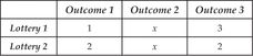
Lottery Winnings
This describes the amount of money you get paid based on the outcome, or more accurately it describes many different possible lotteries, depending on the amount x you get if outcome 2 occurs. Do you prefer Lottery 1 or Lottery 2? Does it depend on x? Economists imagine that x doesn’t really matter to most people since you get the same x in outcome 2 in both lotteries. So really the choice is between 1 in Outcome 1 with 3 in Outcome 3 versus 2 in both outcomes. If you prefer lottery 2 for x = 2 then we suspect you will prefer it when x = 5 or some other number. This is called the independence of irrelevant alternatives or just the independence axiom: the result of Outcome 2 is irrelevant as you get the same amount in both lotteries.
Finally, suppose that given three outcomes A, B and C, where A is better than B is better than C, we can find some probabilities between A and C that would leave you indifferent to B. That is, since B is in between A and C in your ranking, if you had a low enough probability of A and high enough probability of C, you should be willing to take that in place of B and vice versa. This is called the continuity axiom.
If your lottery preferences satisfy all of these axioms: reduction of compound lotteries, transitivity, independence and continuity, then it is possible to give a mathematical description of your preferences by means of a utility function – often called the Von-Neumann Morgenstern utility function4 – that assigns utility numbers to outcomes and in which you rank lotteries by the expected value – the probability weighted average – of those utility numbers. That in brief is expected utility theory.
Most people find the axioms relatively plausible – few argue that they wish to behave otherwise: for example that there are lotteries A better than B better than C, but really C is better than A. Or that they would reverse their choices based on irrelevant alternatives. Unfortunately, when given real (or hypothetical) choices, people do violate the axioms. This was first pointed out by the economist Maurice Allais in 1953.
In the original version of the Allais paradox you are offered a (hypothetical for obvious reasons) choice between getting $1 million for sure versus a risky choice giving $1 million with 89% probability, $5 million with 10% probability and nothing with 1% probability. Most people choose the $1 million for sure. You are then offered an alternative scenario in which you choose between an 11% chance of $1 million (and 89% of nothing); or a 10% chance of $5 million. Most people prefer the 10% chance of $5 million. Unluckily the only difference between the two scenarios lies in an irrelevant alternative: in the first scenario there are 89 cases where you get $1 million in both lotteries and the second scenario differs only in that in those same 89 cases you get nothing. Therefore, if you choose the sure thing in Scenario 1 and the $5 million in Scenario 2, you have violated the independence axiom.
I don’t know if this example will work for you but give it a shot. I give this to my undergraduate students in class, and it worked well for years. Then one year – the year that all the students said that their life ambition was to become rich by selling commercial real estate – it stopped working because nobody chose the $1 million for sure in the first scenario. What I did was to – understanding that $1 million isn’t worth what it was in 1953, especially not to a group of people hoping to earn much more than that – change the millions to billions and all was well. Thus, if the numbers above don’t work for you, try it again with billions.
There are a number of possible explanations of the Allais paradox examined over the years by economists. Rubinstein [1988] and Leland [1994] suggest people might focus on the fact that a 1% chance of getting nothing is quite different than a 0% chance, but be less cognizant of the difference between 89% and 90%, while Andreoni and Sprenger [2010] presume that people perceive the probabilities zero and one quite differently than other probabilities. Machina [1982] suggests a systematic non-linearity of preference in probabilities. Behavioral economists and psychologists have their own theory – prospect theory – that we will come to shortly.
Risk Preferences: the Rabin Paradox
The Allais paradox is not widely viewed as an important deviation from the theory of expected utility by economists. The reason is that to get the paradox the numbers in the gambles must be very carefully chosen. As I mentioned, with my undergraduates the paradox vanished one day because the value of a million fell enough that they decided that it was worth giving up a sure million for a 10% chance at $5 million and an 89% chance of the $1 million despite the 1% risk of getting nothing. If we don’t craft the numbers just right, we don’t get a reversal. Typical economic choices don’t involve such carefully chosen numbers, so the paradox does not have much practical import.
A much more significant puzzle is that raised by Matthew Rabin in Econometrica in 2000. To explain that puzzle we must examine the most important application of expected utility theory – the idea of risk aversion. There are few terms more misused than this one – even by economists who should know better. People say “I don’t buy tickets in the state lottery because I am risk averse.” As it happens for every dollar you bet in the state lottery you will win on average about 50 cents.5 That isn’t risk aversion. Risk aversion means that if for every dollar you bet in the state lottery you will win on average more than one dollar, you still don’t bet because of the risk of losing. For example, I hold up a $100 bill and a $10 bill and offer to flip a coin: if it is heads you get the $110; if you lose you give me $100. If you say no, then you are risk averse. This is because the expected value of a 50% chance of $110 and a 50% chance of -$100 is five dollars. If a gamble has a positive expected value and you reject it you are risk averse. By contrast, if it has a negative expected value and you accept it you are risk loving. So in the case of the state lottery, we can say that someone who purchases tickets is risk loving, but we can’t say whether or not someone who doesn’t purchase tickets is risk loving or risk averse.
Turning back to the win $110 lose $100 with equal chance, if you are just on the margin between accepting and rejecting the bet, then we say you have a risk premium of $5 because you are willing to give up an expected gain of that amount to avoid the uncertainty of the gamble. Economists have a measure of how risk averse people are called the coefficient of relative risk aversion. Exactly what this is can be a bit complicated to explain, but the key idea is this: let us measure the stakes by the proportion of your lifetime wealth. For example if you are worth a million dollars, then a loss of $100,000 represents a 10% loss. The key feature of the coefficient of relative risk aversion is that if my coefficient is twice your coefficient, then for any given gamble, I will demand twice the risk premium you do. If we have the same wealth, and your risk premium is $5 for the win $110 lose $100 with equal probability, then my risk premium is $10, meaning in addition to foregoing the gamble and giving up $5, I’d be willing to pay an extra $5 to avoid it.
With these tools under our belt, let me give my own version of the Rabin paradox – drawn from years of watching experimental papers presented in which coefficients of relative risk were measured – and in which the presenters never once mentioning that the results are nonsense by three orders of magnitude. Suppose that your lifetime wealth is $860,000 which is about the median in the United States. Suppose also that you are indifferent between a 70%:30% chance of $40 and $32 and the same chances of $77 and $2 – which many people are in the laboratory (Holt and Laury [2002]). Then your coefficient of relative risk aversion is 27,950. If this sounds like a big number, it is. One important puzzle much studied by economists is why the rate of return on stocks is so much higher than on bonds, given that stocks are not all that much riskier. One thing we can do is to calculate how risk averse a person would be who is on the margin between buying stocks (an S&P 500 index mutual fund) and U.S. government bonds – a situation many of us are in. The answer is that the corresponding coefficient of relative risk aversion is 8.84. This is over three orders of magnitude different than the answer we find in the laboratory.
This enormously higher risk aversion for small stakes gambles than for large stakes gambles was documented in a clever way by Matt Rabin. It poses an enormous challenge for economics and one that by and large economists have not attempted to address. It flavors laboratory research, which sometimes take as given the relatively low risk aversion observed for large stakes gambles and proceeds to ignore the fact that we know that for the small stakes gambles we observe in the laboratory people are far more risk averse. It poses also a difficult theoretical challenge since the existing theory of expected utility is not able to explain this enormous discrepancy. While several explanations have been offered, none has achieved widespread acceptance. The most widely used theory that can potentially explain the discrepancy is the psychological theory called prospect theory – which however is not widely used by economists.
Risk Preferences: Prospect Theory to the Rescue?
Because of the Allais and Rabin paradoxes psychologists widely regard the expected utility theory used by economists as nuts. As mentioned they also have a serious alternative called prospect theory. Prospect theory differs from expected utility theory in two ways. First, it allows for what is called a probability distortion. This says that people tend to exaggerate low probabilities. Second, it incorporates what is called a reference point. This says that people are not concerned with the effect of a gamble on some sort of measure of overall well-being, but rather with the gains and losses relative to a reference point. If I seem vague about what the reference point is there is a reason: it is treated as an unknown value that varies from setting to setting in an unexplained manner. From the perspective of an economist this is a bug that renders the theory unusable. A theory that says behavior depends on some unknown variable that changes in an unexplained way does not make very useful predictions.
Let us start with the part of prospect theory that says that people over-weight low probabilities and under-weight high probabilities. Is this true? Bruhin, Fehr-Duda and Epper [2007] (economists, by the way) carry out a careful experimental study to find what the probability weighting function might be. Suppose that Pi is the chance of winning one of two prizes xi ≥ 0, where i is the generic name for prize 1 and prize 2. For the mathematically inclined – and if you think you can do behavioral economics without mathematics, think again – they find that for many people if we define a utility function over the probability and prizes by the formula
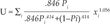
then the gambling behavior of these people is described by picking the gamble that yields the highest numerical value of the utility.
One issue with theories, however, is that they make a range of predictions – not only in the laboratory, but also outside the laboratory. Which would you rather have?
A. $5,000 for sure (or)
B. a 50–50 coin-flip between $9,700 dollars and nothing
People I have asked all prefer alternative A. However the utility function above yields a higher numerical value for option B, thus according to Bruhin, Fehr-Duda, and Epper, such an individual will choose B. As the “typical” person doesn’t do this, prospect theory is not without its own paradoxes.
To pursue this further, prospect theory is motivated in part by the Allais paradox. Recall that there are two scenarios: in Scenario 1 you choose between a certain $1 million and a lottery offering a nothing with a 1% probability, $1 million with an 89% probability, and $5 million with a 10% probability. Most people choose the certain $1 million. In Scenario 2 you are offered the choice between two lotteries. The first lottery offers nothing with 89% probability and $1 million with 11% probability, while the second offers nothing with 90% probability and $5 million with 10% probability. Here most people choose the 10% chance of $5 million. Prospect theory offers a possible resolution of this paradox because smaller probabilities are exaggerated, making the first choice relatively unattractive in Scenario 1, but not so much so in Scenario 2. Unfortunately the Bruhin, Fehr-Duda and Epper [2007] utility function above while explaining the laboratory data also predicts that the “typical” person will not exhibit the Allais paradox.
Prospect theory is largely an empirical and experimental based theory. Many of the experiments on which it is based are for hypothetical money or for very small amounts of money. A question that is always important in this context – the more so given the Rabin paradox – is how the laboratory results reflect on real behavior. Indeed, it turns out that the empirical research underlying prospect theory is a case study in how problematic this can be. One of the main hypotheses in prospect theory is that people are risk averse for gains, but risk loving for losses. However: it isn’t all that easy to present people with the possibility of losses in the laboratory. We can’t easily force people to engage in gambles that involve them losing money. If we start them off with an initial stake that they can lose, we have to worry about the impact that stake has on their “reference point.” As a result experiments involving gains have typically been done for larger stakes than experiments involving losses and indeed most of the losses have been hypothetical rather than real. That raises the possibility that people aren’t risk averse for gains and risk loving for losses at all, but rather that they are risk loving for small (real) stakes and risk averse for (real) large stakes – quite different than is assumed in prospect theory.
In 2006 two clever investigators, Bosch-Domenech and Silvestre examined the possibility that risk aversion and risk loving are driven by the stakes rather than by gains and losses. To allow the possibility of substantial losses, they endowed subjects with money in one experiment, then – to avoid any possible effect of having given them money – they conducted the gambles in a second experiment several months later. What they found is that prospect theory is wrong: risk aversion and risk loving are in fact driven by stakes and not by losses and gains.
Interestingly there is evidence outside the laboratory that people are risk loving with respect to losses. For example: in the recent crisis, and historically as well, bankers have always appeared to be willing to gamble a small probability of a large loss for a modest increase in the average return. Prospect theory appears to predict this kind of behavior, and indeed we find Godlewski in 2007 proposing exactly this possibility. There are two problems with this analysis. First, as we just pointed out, laboratory data does not show that people are risk loving for substantial losses. Second, standard expected utility theory predicts that bankers should gamble on losses.
Have you heard of the “hail Mary pass” in football? That’s when a team just throws the ball wildly down the field gambling that somehow they will get lucky and someone on their team will grab it and score. Usually the opposite happens, the other team grabs it and scores instead. Of course the reason teams do this is because the game is ending, they are behind, and it is unlikely that they will win the game. Losing the game by 13 points rather than 6 doesn’t matter, and the only way they can hope to win is by gambling. Bankers face a similar situation – not that their game is about to end, but rather that their loss is truncated. If they win, they get to pocket a nice commission. If they lose – then the government steps in and bails them out. When bigger losses don’t matter – either because it doesn’t matter how much you lose the game by or because the government will bail you out no matter how great the loss – expected utility theory – and common sense – indicate that gambling is a good idea.
This notion that prospect theory is somehow needed to explain the gambling behavior of bankers is once again behavioral economics at its worst. Expected utility theory provides a simple and obvious explanation for what we see. Prospect theory is not needed here.
In summary, expected utility theory has its paradoxes. Prospect theory is an effort to explain those paradoxes. Unfortunately when subject to the same scrutiny as expected utility theory it has its own equally serious paradoxes.
To give credit to psychologists – the fact that prospect theory allows attitudes towards risk to depend on the context (or a reference point) at least attempts to come to grips with the Rabin paradox. I do not know of any way to explain the wildly different attitudes towards large and small risks without some model of context dependence. Unfortunately the lack of an adequate theory of the reference point renders prospect theory useless for economists.6
Risk Preferences: How Research in Economics Works
Critics of economic theory seem to be under the impression that economists are wedded to elegant models and oblivious to any facts that might fly in the face of those models. Nothing could be less true. A case study involving a famous and important paradox helps to illustrate the point.
In 1981 Shiller gathered over 100 years of data on stock market returns, bond returns, and consumption data. He observed that under rational expectations the price of stocks is supposed to be a weighted average of future dividend payments. For any fixed weights this implies that prices should fluctuate less than dividends: something that is not true in the data. Unfortunately for this calculation – the so called excess volatility puzzle – this is only true for fixed weights, and theory and evidence suggests that the weights fluctuate enough to cause the observed fluctuations in prices. Several years later in 1985 Mehra and Prescott pointed out a rather more serious puzzle in Shiller’s data, the equity premium puzzle.
If we look at the returns in Shiller’s data, properly adjusted for inflation, we find that safe government bonds had a return of about 1.9%, while stocks had a much higher return of 7.5%.7 This of course isn’t much of a puzzle: it is much easier to lose your shirt by investing in stocks than in bonds, as many investors recently have had the misfortunate to verify. In fact, we can measure relatively well the amount of risk involved in stock investment: in the Shiller data a measure of the risk is the standard error of the stock return, which is 18.1%. This means that roughly 68% of the time stock returns lie between 7.5% – 18.1% = –10.6% and 7.5% + 18.1% = 25.6%. That seems pretty risky, but when we apply our tool of relative risk aversion to ask how risk averse an individual would have to be to be indifferent between investing in stocks and bonds, we find that it should be around 8.84, which is the result we reported before in our discussion of the Rabin paradox. That number is pretty small compared to the laboratory value of 27,950, but never-the-less it turns out to be too large.
What can we mean by too large? After all, people are how risk averse they are. Perhaps their risk aversion is indeed 8.84. However, the coefficient of risk aversion governs behavior in a number of domains, so it may be that their behavior in other domains is inconsistent with 8.84 for stocks and bonds. And indeed there are two major problems with this number. First, as pointed out by Boldrin and Levine [2001], any coefficient of relative risk aversion bigger than one implies that the stock market prices respond to bad news by going up – the opposite of what we observe. Second, as observed by Mehra and Prescott, in standard theory the coefficient of relative risk aversion determines our willingness to save. In particular in the same Shiller data used to compute stock and bond returns, real per capita consumption in the United States grew on average 1.8% per year. It turns out that an individual with a coefficient of relative risk aversion of 8.84 faced with a 1.9% return on bonds would not wish their consumption to grow nearly this fast: they would wish to borrow heavily against the future. It is this contradiction between the amount of risk aversion observed in choosing between stocks and bonds and savings behavior that is the equity premium puzzle.
So what have economists done in response to this puzzle? Built ever more elegant and less relevant models? They can’t easily be accused of ignoring it: a citation count on Google Scholar8 shows 3,726 follow-on papers to Mehra and Prescott. Many of these papers were published in top journals such as the Journal of Political Economy, the American Economic Review and Econometrica. Did anyone turn to prospect theory? Of course that was tried – and discarded along with various other approaches for a very simple reason – because it didn’t help explain the puzzle. One can fairly easily find various papers by “behavioral economists” claiming that the puzzle was solved by various means including prospect theory, however what these papers have in common is that they don’t recognize that the puzzle involves not the fact that people are very risk averse, but rather that their risk aversion in the stock/bond decision contradicts their behavior in other domains.
What is striking about this is that prospect theory appears to have at its core an idea that might help explain the equity premium puzzled: the idea of a reference point that leads to different behavior in different domains. Unfortunately prospect theory’s reference point doesn’t say anything about the stock/bond domain versus the savings domain. In 1990, fortunately, Constantinides (an economist) produced a model of habit formation that not only provided a reference point governing risk behavior and intertemporal behavior, but provided a clear theory of what determined the reference point. The idea is a simple and intuitive one: as we consume at a particular level it becomes a habit, and as the novelty wears off, we need increases in consumption to feed our utility. Conversely, declines in consumption are very difficult to bear, having habituated ourselves to a higher level. This makes us very risk averse. At the same time it causes us to demand ever growing consumption as we race to get ahead of our habit.
One question – rarely asked by behavioral economists – is whether such a substantial change in assumptions about individual behavior might – while explaining one thing, namely the equity premium – might also unexplain other things. For example, we can explain around 50% of business cycle fluctuations using a straightforward model of growth – without habit formation. Naturally economists have examined whether the habit formation model has unpleasant as well as pleasant implications. One reason the model has become popular is because in 2001 Boldrin, Christiano and Fisher showed that introducing habit formation into a real business cycle model if anything improves its ability to explain economic fluctuations.
It is worth mentioning also a related class of models called consumption lock-in models. These models are technically a bit different than habit formation models but have a very similar flavor: they assume that after you choose a particular level of consumption it is costly to adjust it right away, either up or down. These models also date back to 1990 when they were introduced by Grossman and Laroque. As Grossman and Laroque argued, while standard theory says that people ought to adjust their consumption in response to changes in stock market prices, nobody is terribly likely to sell their house and buy a slightly larger or smaller one in response to a modest change in stock prices (although they might skimp a bit on maintenance if prices fall).
In 2001 Gabaix and Laibson produced a very simple version of the consumption lock-in model showing that a lock-in of about a year and a half is what is needed to explain the equity premium. One advantage of these models over habit formation is that when combined with a model of self-control they can also produce the Rabin paradox: this was shown by Fudenberg and Levine in 2006.
The key thing to note is that these models were a response to a real problem that concerned economists. None of them are “behavioral” in the sense of Akerlof or Ariely, and indeed, nobody has come yet up with a sensible explanation of asset prices based on irrationality. Moreover: there is no shortage of explanations of the equity premium – explanations ranging from taxes to problems with the way the data were chosen have been proposed. Our problem is a surfeit of riches: we have too many explanations of the equity premium puzzle, not too few.
Notes
1 This experimental result is confirmed by Weber and Chapman [2005], and discussed in Halevy [2008], who proposed an objective function that is consistent with these choices. Note that the experiment was in Dutch Florins. I converted from Dutch Florins to U.S. Dollars using an exchange rate typical of the early 1990s of 1.75 Florins per Dollar.
2 The sample consists of 60 individuals.
3 Sample sizes are in parentheses.
4 Their 1944 book systematically developed the theory first proposed by Bernoulli.
5 See for example Garrett and Sobel [1999].
6 Plott in his 1996 review of one of Kahneman’s many attacks on standard economics carefully examines why his proposed theory is useless for economists.
7 Stock returns are measured by returns on the Standard and Poor’s 500 index. This is the broadest measure of stock returns that is available over such a long period of time.
8 Search conducted October 23, 2011 at 3:32 AM Pacific Standard Time.