


II. The general advice in the Key Stage 3 programme of study
Schools will naturally try to implement and adapt the published programme as it stands. It is therefore important to decide
•when it is safe simply to copy what is listed;
•when the given list of topics needs to be reordered or supplemented in some way; and
•when there are strong mathematical reasons to reinterpret an official requirement (and to clarify in one’s own mind why it needs to be reinterpreted).
Hence the remaining sections of this book are presented in the form of a line-by-line commentary (where comment seems needed) on the published programme. The present part, Part II, concentrates
•on the Aims etc. which appear on page 2 of the published programmes of study (Section 1 below), and
•on the broad expectations discussed in the section headed Working mathematically on pages 4 and 5 of the published programmes of study (Section 2 below).
Mathematics is an interconnected subject in which pupils need to be able to move fluently between [different] representations and mathematical ideas.
Elementary mathematics derives its power from the way a simple idea sometimes has other interpretations, and from the way simple ideas from different domains can be combined to deliver more than one might expect. The published programme of study does not always make it easy to identify these connections and interactions. Hence it is important to consider how to sequence and to link the listed material in a way that clarifies and develops the interdependencies between topics and ideas.
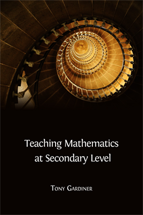
For example, if we consider the most familiar idea of all—namely ‘place value’—schools may recognise the need to reinforce:
•how the place value notation for integers works, and how it extends to decimals;
•that it does so in a way that links
–the more familiar positive powers of 10 (tens, hundreds, thousands),
–with 100 = 1 (the ‘units’ or ‘1s’ place), and
–with negative powers of 10 (for places to the right of the decimal point);
•the fact that powers of 10 multiply together in a way that foreshadows the index laws for general powers;
•that the written algorithms of column arithmetic, which were developed in primary school for integers, extend naturally to decimals—giving plenty of opportunity to reinforce both the procedures themselves and why they work, and hence to strengthen pupils’ sense of ‘place value’.
Schools will benefit from identifying such recurring themes and important connections for themselves, and from organising the required Key Stage 3 content so that pupils come to appreciate these themes and connections. Some of these are very basic. The next ten bullet points indicate a few selected examples to illustrate the need
–to consider each of the requirements listed in the programme of study,
–to decide what links need to be explicitly mentioned, and
–where possible to include these in any scheme of work.
•The way work with pure numbers (that is, numbers like 1, 23,  , or −67.8, stripped of any units), and the arithmetic of integers and decimals, links to simple applications—where purely numerical calculations allow one to solve problems involving measures, and to make sense of, and solve, all sorts of ‘word problems’.
•The way multiplication and division of decimals and fractions hold the key to routinely solving almost any problem involving rates, or percentages, or ratios, or proportion.
•The way blind calculation gives way to simplification and “structural arithmetic”, which links naturally to effective calculation in algebra.
•The way “I’m thinking of a number …” problems should at first be tackled without algebra (as ‘inverse mental arithmetic’), but can later be formulated as a simple equation in one unknown, then routinely solved.
•The way any linear equation in one unknown x reduces to ax + b = 0, with solution x =  ; and any linear inequality in one unknown x reduces either to
(i)ax + b > 0 (or ax + b ⩾ 0) with a > 0, having solution x > (or x ⩾ )—i.e. a ‘half-line’; or alternatively to
(ii)ax + b < 0 (or ax + b ⩽ 0) with a > 0.
•The way any linear equation y = mx + c in two unknowns x, y corresponds geometrically to the set of all points (x, y) on a straight line, that the line divides the plane into two ‘half-planes’, and that the solutions of the corresponding linear inequality (y > mx + c, or y ⩾ mx + c) correspond to the set of all points (x, y) in one of these two half-planes.
•The fact that two simultaneous linear equations can be solved exactly, and that the solution is the point of intersection of the two lines corresponding to the linear equations (provided the two lines meet).
•The way short and long division (combined with a little algebra) shows that fractions correspond precisely to terminating or recurring decimals.
•The way the basic property of parallel lines forces the sum of the angles in a triangle to be equal to the sum of the angles at a point on a straight line.
•The way the congruence criterion and the parallel criterion allow us to justify the standard ruler and compass constructions, and to prove the basic facts about areas (of parallelograms and triangles), which lead to a proof that in any right angled triangle the square on the hypotenuse is miraculously equal to the sum of the squares on the other two sides, which then links with coordinate geometry by allowing us to calculate exactly the distance between any two given points in 2D or in 3D.
Pupils should build on Key Stage 2
This is excellent advice—provided it is suitably interpreted. Key Stage 3 has to start out from pupils’ experience at Key Stage 2. But this prior experience also needs to be revisited and developed in fresh ways if it is to be used as a reliable foundation for further work. In commenting on this principle, we consider one example in modest detail (1.2.1), then digress to make three important general points (1.2.2–1.2.4), indicate some further examples more briefly (1.2.5), and end with a gentle warning about the likely impact of the Key Stage 2 programme of study on Key Stage 3 (1.2.6).
1.2.1Mental calculation work should not end with Key Stage 2. It should continue in Year 7, but should increasingly use what pupils know in a way that exploits structure, rather than calculating blindly.
•Pupils need to learn to be on the look-out for ways of extracting 10s and 100s in additions such as
73 + 48 + 27 = …;
or in multiplications such as
14 × 45 = 7 × (2 × 5) × 9 = 630,
or
75 × 28 = 3 × (25 × 4) × 7 = 2100.
•Decimal calculations (such as 7 × 0.8 = …, and 12 × 1.2 = …, and 0.7 × 0.08 = …, and 1.2 × 1.2 = …) should be routinely related to their familiar integer equivalents, exploiting opportunities to reflect on how multiplying and dividing by powers of 10 affects the decimal point.
•Common factors among a list of added terms should be seen as an opportunity to ‘group’ using the distributive law, as in
17 × 23 + 17 × 7 = 17 × (23 + 7) = 17 × 30,
rather than to calculate the left hand side blindly. In general, common factors among terms which are to be added or subtracted, multiplied or divided, should be seen as an opportunity to simplify and to cancel.
•Lots of simple work involving fractions should include (a) switching to common denominators (by scaling up both numerator and denominator) in order to simplify the arithmetic, and (b) moving in the opposite direction when using cancellation to simplify fractions.
Written calculation with integers also needs to be strengthened and extended to decimals—but we shall have more to say on this in Section 1.2.5 below.
1.2.2In Part I we saw clear evidence (in the two Ofsted reports) of the unfortunate consequences when a Key Stage seeks to maximise performance on immediately impending assessments, and forgets
that our primary responsibility is always to prepare pupils for the Key Stages that follow.
Pressure to “achieve” in the short-term often encourages pupils to become dependent on (and teachers to allow) ‘backward-looking’ methods that deliver answers in easy cases, but which sooner or later become an obstacle to progress. Hence any internal scheme of work needs to make a clear distinction between
(a)backward-looking methods that get answers in the short-term, but which trap pupils in old ways of working (as with finger counting, or idiosyncratic calculation methods, or reducing multiplication to repeated addition, or modelling questions about fractions in terms of pizzas—all of which may have transitional value, but which are known to block later progress if they become too strongly embedded), and
(b)forward-looking methods, that may seem unnecessary if the perceived goal is merely to get answers to simple problems at a given stage, but which are important because of the way they reflect the inner structure of elementary mathematics, and are often essential for progress at the next stage.
It is not easy for a mere listing of curriculum content to capture this crucial distinction. An effective primary school is one whose pupils are taught in such a way that allows them to flourish at Key Stages 3 and 4. Similarly, effective teaching at Key Stage 3 prepares the ground for, and leads to solid achievement at Key Stage 4 and beyond. Insofar as the revised programme of study incorporates this idea, it tends to do so in ways that are not immediately apparent, so we shall occasionally comment on how Key Stage 3 material impacts on mathematics at Key Stage 4 and beyond.
1.2.3The previous subsection drew attention to the distinction between backward-looking and forward-looking methods. Another important distinction is that between
•a direct operation (such as addition, or multiplication, or evaluating powers, or multiplying out brackets), and
•the associated inverse operation (such as subtraction, or division, or identifying roots, or factorising).
The distinction may be easier to appreciate if we consider a strictly artificial example—namely the “24 game”. Four numbers are given, and each is to be used once. These four numbers may be combined using any three operations chosen from the four rules (with brackets as required), with the goal being to “make 24”.
If one is given the starting numbers “3, 3, 4, 4”, then one scarcely notices the distinction between
•a ‘direct’ calculation (such as “Work out (3 × 4) + (3 × 4) = …”), and
•the ‘inverse’ challenge of having to “invent for oneself a way to make 24” (let’s try “(3 + 3) + (4 × 4) = 22”— not quite; or “(3 × 3) + (4 × 4) = 25”—nearly; or “(3 × 4) + (3 × 4) = …”).
When faced with the inverse challenge to “make 24 using 3, 3, 4, 4”, it is almost as easy to dream up a combination that works as it is to evaluate the expression once it has been invented. But
•evaluating the answer of a given sum is a direct, or mechanical, process, whereas
•juggling possibilities to come up with a calculation which produces the required answer of “24” is an inverse operation, which is far from mechanical (even if in this case it is rather easy).
The distinction between direct and inverse operations becomes slightly clearer if the given numbers are “3, 3, 5, 5”. Here the inverse task of coming up with a sum that delivers the required answer of “24” is significantly harder. The relevant tools are the direct processes of arithmetic—except that it is not clear which to use, so one has to scan what one knows, and select approaches which seem to be the most promising. It is precisely this willingness to juggle intelligently with numbers, and to think flexibly with simple ideas that is needed in many everyday applications. But once one is told what calculation to carry out, then the direct calculation “(5 × 5) – (3 ÷ 3)” is entirely routine.
This distinction between the direct operation (which is straightforward, and which requires only that one should implement a given calculation to check that the answer is equal to “24”), and the inverse operation (which is much harder, and which here requires us to invent a sum that has the required answer “24”), becomes markedly more clear if one is given the starting numbers 3, 3, 6, 6, and is left to find a way to “make 24” (or if one is given the starting numbers 3, 3, 7, 7; or 3, 3, 8, 8).
To sum up: the reasons why this distinction is important are that
•almost every mathematical technique one learns comes initially in a direct, or mechanical, form, but leads naturally to inverse problems (as addition leads naturally to subtraction);
•inverse problems are usually much more demanding than their direct cousins;
•mastery of the inverse form depends on a prior robust mastery of the direct form;
•but in the long run, it is the inverse operation which is generally more important.
Those who complain that pupils, or school leavers, cannot “use” what they are supposed to know, often fail to notice that what pupils have been taught (and what has been assessed) has usually focused on direct procedures, whereas what is required is the ability to think more flexibly when faced with some kind of inverse problem. Inverse problems often come in different forms, or variations something that has been a focal point of the recent teacher exchanges with Shanghai, where the idea of “exercises with variation” has emerged as a recurring didactical theme
Given this, one might expect formal assessments to include a strong focus on ensuring mastery of the many inverse operations and the ability to solve the standard inverse problems in elementary school mathematics. In reality, inverse processes have been neglected, or (worse) have been distorted by providing ready-made intermediate stepping stones that reduce every inverse problem to a sequence of direct steps. Why is this?
Direct operations are relatively easy to teach, and to assess. The associated inverse operations may be more important, but they are harder to assess. Inverse problems are more demanding, and cannot be reduced to deterministic methods. So they give rise to low scores, and they do so in a way that is hard to predict. This makes them distinctly awkward for those who devise test items within a target-driven and test-driven culture, where the assessors may be contractually obliged to return predictable results, and to avoid low scores. Hence, if such problems are set at all, they are usually adapted in some way to make pupil performance more predictable (for example, by breaking down the unpredictable inverse problem into a more manageable sequence of steps—each of which is essentially a routine direct task).
Teachers need to recognise the importance of such problems for pupils’ subsequent progress, and then devote sufficient time to them for pupils to achieve a degree of mastery. But it would obviously help if assessments regularly required, and rewarded, such mastery!
1.2.4The bald listing of content in the official programme of study is rather dry and formal—focusing on “what” rather than “how”. In one sense, this emphasis is healthy. But it ignores the essential interplay between content and didactics.
Procedural fluency is rightly stressed. But this emphasis is too often repeated in isolation—as though a robust grasp of place value (for example) will emerge spontaneously as a result of banging on about fluency in specified procedures. It won’t. So something more is needed. If it is to serve as a useful guide, a content list or programme of study needs to be constructed in a way that indicates, and supports, a clear underlying “didactical architecture”. In contrast, the given programme of study routinely misses the opportunity to convey key central principles (such as the contrast between backward-looking and forward-looking methods, or between direct and inverse operations), and important details (such as the key didactical stages which can lead from:
(a)talking about “half a pint” or “half an hour” in Year 2, to competence with the arithmetic of fractions in Year 9; or
(b)from meeting negative quantities for the first time in Key Stage 2, to calculating freely with negative numbers, and simplifying expressions which combine subtraction and minus signs in algebra at Key Stage 3/4).
1.2.5In early Key Stage 3 we need to reinforce Key Stage 2 work on the familiar written arithmetical procedures for integers in order to extend them to more serious long multiplication, to division, and to decimals. Column arithmetic for integers provides an excellent opportunity to cement number bonds and multiplication tables. It also develops the ability to carry out a sequence of simple steps completely reliably. The extension of these procedures to decimals provides fresh opportunities to address ‘place value’. At the simplest level, pupils need to understand why it is essential to align the units and tens “places” when carrying out column addition and subtraction of integers, so that the requirement to align the decimal points when adding and subtracting decimals is recognised as being essential (see example 1.2.2C “42.65 + 5.748 = …” in Part III). The logic of short and long multiplication will also need to be clarified before these procedures are extended to decimals. Integer arithmetic (including mental arithmetic in both direct and inverse forms with all variations) also needs to be in good shape before we extend integer arithmetic to fractions.
The extension of long multiplication and division to decimals may need to be slightly delayed. When they are addressed, pupils need first to know how the decimal point behaves under multiplication and division by powers of 10, so that they can understand how this allows multiplication and division of decimals to be transformed into integer multiplication and division.
Short and long division develop the inverse of multiplication, in that they require pupils to use what they know about multiplication in a flexible way. When asked to divide 17 onto 918, the initial inverse question:
“How many times does 17 go into 91? And what is the remainder?”
requires greater mental agility than the two direct questions:
“What is 17 × 5?”, and “What is 91 − 85?”.
Short and long division also require pupils to string together a chain of steps, each of which is accessible, but where the whole chain has to be implemented 100% reliably for the process as a whole to succeed. And the power of the process becomes apparent when one discovers how it extends naturally to allow division of decimals. Later the division process helps to establish the remarkable connection between fractions and decimals.
Some pupils will benefit from the challenge of tackling (or extending their prior facility with) serious long division. This topic is listed in Key Stage 2 for all pupils. It is unclear what effect this may have; but we may well find that serious long division is appropriate for only around half of the cohort, even at Key Stage 3.
1.2.6In exhorting teachers at Key Stage 3 to “build on Key Stage 2” it is only fair to mention that the Key Stage 2 programme of study may prove problematic in some respects. A preliminary indication of the extent of this difficulty may be gleaned from an earlier paper.5 In particular
•a significant amount of material has been included at Key Stage 2 in a way that is likely to prove premature; and
•some of the listed topics which are entirely appropriate in Year 5 and 6 have been specified rather poorly.
Hence one can anticipate that many pupils entering Key Stage 3 will have at best a superficial grasp of some of the listed content from Key Stage 2.
Among the listed topics that are inappropriate and unnecessary in Year 6, many are implicit in the early Key Stage 3 programme of study, so could be safely delayed until Year 7. Some primary schools may recognise this and concentrate on more age-appropriate material—leaving other content to be treated more effectively at Key Stage 3. But many schools will go by the book and will try to cover whatever is listed—with predictable consequences. For both groups, this problematic material will need to be revisited at Key Stage 3 in order to establish a secure platform for progression. Examples of topics which may have been ‘covered’ at Key Stage 2, but which will need serious attention in Years 7 and 8 include:
•the extension of place value to decimals;
•work with measures—especially compound measures;
•the arithmetic of fractions;
•ratio and proportion;
•the use of negative numbers;
•work with coordinates in all four quadrants;
•simple algebra.
Decisions about progression should be based on the security of pupils’ understanding and their readiness to progress to the next stage.
Secondary schools will need to know how this excellent principle of “readiness to progress” has been handled at Key Stage 2. We give just one example of many.
There is a general welcome for the requirement that pupils should learn (i.e. know, and be able to use) their tables. But there is unanimity that this will not be achieved by the end of Year 4 as specified in the official programme of study, and that a more realistic objective may be to expect most pupils to achieve this by the end of Year 5 or Year 6. Hence material listed in Year 5 and Year 6 that depends on ‘prior mastery of tables’ will not be accessible at the expected stage, so will prove unrealistic at that level. (For example, until tables are secure, one is limited in what one can achieve in factorising integers, finding HCFs, working with prime numbers, with short division and long division, with squares and cubes, with equivalent fractions and with cancellation.)
If primary schools feel obliged to try to teach inappropriately ambitious material purely because it is officially listed, this will lead to problems that are entirely avoidable. Thus secondary schools may have to encourage their feeder primary schools to trust their professional judgement in such matters, and to recognise those aspects of the Year 6 programme where work should remain ‘preparatory’, with a serious treatment being delayed until Year 7.
Some of the material that is listed in Key Stage 2 seems inappropriate at that level—partly because we know that it is hard to teach it well even at Key Stage 3. For example, it may make sense at Key Stage 2 to use symbols to summarise familiar formulae: such as re-writing the verbal equation
“(area of a rectangle) = (length times breadth)” as “A = l × b”.
However, it would be premature to expect most primary pupils to learn more serious elementary algebra (and most primary teachers are in no position to teach it effectively). And while there is every reason to engage pupils at Key Stage 2 in tackling “I’m thinking of a number …” problems, they are best addressed at that age by using ‘inverse mental arithmetic’: that is, where the missing number is discovered by using intelligent, flexible, inverse mental arithmetic, rather than by prematurely trying to formulate such problems algebraically as equations (as suggested by the official Year 6 programme listed under Algebra).
Even where secondary schools liaise effectively with most of their feeder primaries, they should think carefully—as part of ensuring “readiness to progress”—how to consolidate key ideas and techniques from Key Stage 2 in early Key Stage 3, and should be prepared to clear up misunderstandings that may have arisen as a result of material having been introduced prematurely.
A key application of this crucial principle of “readiness to progress” arises because the Key Stage 3 programme of study is now an explicit part of the GCSE specification. Hence decisions about progress through the Key Stage 3 curriculum are bound up with decisions about future GCSE entry. The Key Stage 4 programme of study states explicitly:
Together the mathematical content set out in the Key Stage 3 and Key Stage 4 programmes of study covers the full range of material contained in the GCSE Mathematics qualification. Wherever it is appropriate, given pupils’ security of understanding and readiness to progress, pupils should be taught the full content set out in this programme of study.
In its understated way this both presents a challenge to teach as much of the listed material as possible to as many pupils as possible, and at the same time leaves considerable scope for teachers to use their professional experience to decide where this aspiration may not be “appropriate”.
Those pupils who should progress comfortably to GCSE Higher tier may be able to swallow the complete Key Stage 3 programme by the end of Year 9. But those who may land up taking Foundation tier GCSE will often benefit from proceeding more slowly through Key Stage 3 in order to establish a solid foundation for those parts of the Key Stage 4 programme which they might subsequently manage to cover, and perhaps master. In other words, schools would seem to be free to interpret the Key Stage 3 programme as part of GCSE, and to allow some material to spill over into Year 10 where this seems appropriate. Those pupils heading for Foundation tier are far more likely to achieve mastery of some of this material if they are allowed to proceed more steadily (e.g. taking four years rather than three), than if they are forced to cover the material prematurely, and then have to repeat it.
Pupils who grasp concepts rapidly should be challenged through being offered rich and sophisticated problems before any acceleration through new content in preparation for Key Stage 4. Those who are not sufficiently fluent should consolidate their understanding, including through additional practice, before moving on.
The second sentence reinforces the comments made at the end of 1.3 above.
The first sentence advises against acceleration. It also highlights the fact that each listed topic can be treated on many levels, and states the important general principle that those who grasp a basic concept should be faced with more challenging variations on the same material before they move ahead. This is an extension of the idea of “readiness to progress”: namely that
before allowing pupils to progress to more advanced topics, we should routinely expect a much deeper understanding on the part of those who might one day proceed further.
At present we routinely let down large numbers of pupils by failing to establish a sufficiently robust mastery of important basic ideas. For example, the very first item under Number (Subject content p. 5: see Part III, section 1) states that pupils should
understand and use place value for decimals, measures and integers of any size.
Other requirements under the sub-heading Number relate to calculating with fractions, working with percentages, and simple algebra. But the evidence is that, even when teaching such basic material we in England have expected far too little—including from our more able pupils. Consider the following items, given to Year 9 pupils in around 50 different countries as part of the major international comparison TIMSS 2011:6
1.4AWhich fraction is equivalent to 0.125?

1.4BWhich number is equal to  ?
?
A: 0.8B: 0.6C: 0.53D: 0.35
1.4C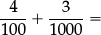
A: 0.043B: 0.1043C: 0.403D: 0.43
1.4DThe fractions  and
and  are equivalent. What is the value of …?
A: 6B: 7C: 11D: 14
1.4EWhich of these number sentences is true?
1.4FWhich shows a correct method for finding  ?
?

1.4GWrite  in decimal form rounded to 2 decimal places.
1.4HSimplify the expression

Show your work.
Success rates are never easy to interpret. But it seems sensible to compare the success rates for Year 9 pupils in England with those in Russia, in Hungary, in the USA, and in Australia rather than with countries from the Far East (for the released items and the corresponding results, see http://timss.bc.edu/timss2011/international-released-items.html). We note that:
•in Russia, children start school only at age 7, and in Hungary at age 6;
•the primary curriculum in Russia may include the idea of fractional parts, and the link with decimals, but calculation with fractions would seem to begin only in secondary school;
•tasks 1.4A–1.4F are multiple-choice questions with just four options, and some of the options could never be obtained as a result of making a mistake (which suggests that the English success rates for 1.4A–1.4C are already embarrassing).
1.4ARussia 86%,USA 76%,Hungary 74%,Australia 67%,England 62%;
1.4BRussia 84%,USA 83%,Australia 70%,Hungary 67%,England 59%;
1.4CRussia 83%,Australia 68%,Hungary 63%,USA 63%,England 57%;
1.4DRussia 62%,USA 55%,Hungary 49%,Australia 45%,England 43%;
1.4ERussia 58%,Hungary 53%,Australia 36%,USA 36%,England 33%;
1.4FRussia 63%,Australia 34%,Hungary 33%,USA 29%,England 28%;
1.4GRussia 39%,Australia 31%,Hungary 29%,USA 29%,England 24%;
1.4HRussia 35%,Hungary 34%,USA 19%,Australia 14%,England 9%.
The implication of these comparisons would seem to be that we in England
•are failing to achieve basic competence even for our more able pupils,
•that we routinely allow (or even encourage) pupils to move on to some “higher level” before basic material has been properly understood, and
•that we need to slow down and routinely use slightly harder and more varied problems to probe and strengthen pupils’ understanding before they move on in this way.
This inference was supported by the recent ICCAMS study which set a sample of 15 year olds in English schools problems that had been used in a similar study in the late 1970s. We give just two examples:
1.4JOn the motorway my car can go 41.8 miles on each gallon of petrol. How many miles can I expect to travel on 8.37 gallons? [Six calculations involving 41.8 and 8.37 were given, and the relevant calculation was to be ‘circled’, not implemented.]
30 years ago 54% of 14 year olds managed to circle 8.37 × 41.8; now only 33% manage this.
1.4KSix tenths written as a decimal is 0.6. How would you write eleven tenths as a decimal?
30 years ago 36% managed to write 1.1; now just 16% of 14 year olds respond correctly.
The message would seem to be clear. We need to do much more work with the most basic material to ensure that pupils grasp the relevant concepts. The last thing our more able pupils need is to be accelerated. They need to slow down, and to strengthen their understanding by tackling harder, and more varied, problems involving the same material as their peers. In particular, notwithstanding the wording of the requirement at the start of Section 1.4, able pupils may need challenges that are surprisingly basic, before they are confronted with material that is “rich and sophisticated”.
The need to replace a philosophy of premature “acceleration” by a strategy of deepening and strengthening was strongly argued in the recent ACME report Raising the bar.7 Any mathematics department which appreciates the importance of avoiding acceleration, but which anticipates being challenged by parents, or by senior management, will find valuable support in this report.
Ministerial advice regarding early GCSE entry has recently changed to reflect the same position. This change in official policy is partly based on overwhelming evidence. The instructive paper,8 which was prepared by the Department for Education for the House of Commons Select Committee, contains some astonishing statistics that should also help to convince sceptical parents and management that acceleration incurs substantial human and resource costs with no evident benefits. Indeed, those who take GCSE early rarely benefit as a result.
This recent shift in policy is in line with the longstanding professional consensus, which was first stated in the analysis and the recommendations of the old report Acceleration or enrichment? (2000).9
This section of the official programme of study contains eighteen bullet points under three headings: Develop fluency, Reason mathematically, and Solve problems. Many of these bullet points appear relatively unproblematic. Hence we restrict our remarks to those requirements that invite comment.
The list of themes referred to in the bullet points under this sub-heading in the official programme of study needs to be further supplemented: e.g. at present there is no mention of measures, or of ratio and proportion, or of word problems, or of geometry.
In recent years those who decided what a typical pupil in England should be expected to learn have downplayed the importance of memorisation, and of fluency. Yet there are all sorts of reasons why we need to learn certain things by heart, and in general to achieve much higher levels of fluency. The word “fluency” is not quite the same as raw speed; but fluency, and the related notions of “learning by heart” and “automaticity”, are useful indicators of understanding and mastery.
Memory contributes significantly to what we are, and to what we can do. We need to be completely on top of that limited collection of basic facts and techniques in terms of which most elementary mathematics can be understood. But we need to memorise far more than this. For example, when tackling an unfamiliar problem, one must be able
•to consider and choose between possible approaches and to compare the alternative intermediate steps in order to assess what seems to be the most promising strategy; and
•to achieve this, the possible steps or techniques need to be robustly internalised and immediately accessible.
Where a pupil struggles to use an idea, or fails to implement a learned procedure quickly and reliably, one can infer either that the ingredient steps need to be strengthened, or that more time needs to be devoted to integrating these steps into an effective method (or both).
When faced with routine inverse problems (such as “simplify  ”; or “factorise x4 − 7x2 + 1”; or “make 24 with 3, 3, 5, 5; or with 3, 3, 6, 6; or with 3, 3, 7, 7; or with 3, 3, 8, 8”), one cannot begin unless the relevant direct facts are immediately to hand. Only then do we have a chance of recognising the relevance of those direct facts.
•We need immediate recognition that 36 = 4 × 9 and 54 = 6 × 9 in order to “simplify  ”.
”.
•Given “3, 3, 5, 5 to make 24” we need to notice immediately that “5 × 5” is “close to 24”, and then that “3 ÷ 3” makes up the difference.
•Later (at Key Stage 4 or beyond), unless the identity
(a2−b2) = (a − b)(a + b)
is second nature, we are most unlikely to notice that
x4 − 7x2 + 1 = (x2 + 1)2 − 9x2 = (x2 − 3x + 1)(x2 + 3x + 1).
That is, we need to memorise enough to enable us to respond flexibly.
What you don’t know by heart, and so can’t access instantly, you can’t use.
This observation applies not only to facts (such as 36 = 4 × 9, and 5 × 5 = 25), but also to procedures. That is, we need to attain fluency in handling a wide range of arithmetical, algebraic, trigonometric and geometrical procedures, so that each new procedure can eventually be exercised automatically, quickly, and accurately. Once this level of automaticity is achieved, the brain is free to focus on those more demanding aspects of a problem that require genuine thought (such as trying to see whether x4 − 7x2 + 1 can be written as a difference of two squares).
2.1.1 [Develop fluency p. 4 ]:
–consolidate their numerical and mathematical capability from Key Stage 2 and extend their understanding of the number system and place value to include decimals, fractions, powers and roots
–select and use appropriate calculation strategies to solve increasingly complex problems
2.1.1.1Consolidating Key Stage 2 work, and choosing and using appropriate calculation strategies should start immediately in Year 7. In particular, mental work should continue, but should move beyond idiosyncratic methods (which may have been quite rightly encouraged at some stage, but which should then have moved on to more efficient methods) towards structural arithmetic in preparation for algebra. (The meaning of “structural arithmetic” is explained briefly in Subsection 2.1.1.2.)
There should also be a continuing thread of word problems, through which pupils learn to extract information from given text and to
“select and use appropriate calculation strategies to solve … problems”.
(What is meant by “word problems” is outlined in Section 2.3 Solve problems, and in particular in Subsection 2.3.3.)
Particular attention should be paid
•to pupils’ facility in working with decimals as an extension of earlier work with integers, including a robust grasp of
(a)the “transition across boundaries” (from 0.9 to 1.0, or from 1.19 to 1.20, or from 2.99 to 3.0, etc.),
(b)multiplying by a suitable power of 10 to change decimals into integers and conversely,
(c)translating decimals into fractions and vice versa,
(d)adding and subtracting fractions and decimals (see the ICCAMS and TIMSS examples 1.4A–1.4K above, and example 1.2.2C in Part III);
•to consolidating long multiplication and short division, and simple long division for integers;
•to extending the standard written arithmetical procedures for integers to decimals (column addition and subtraction, short and long multiplication and short division)—using these procedures to reinforce the idea of place value, and to solve word problems and other problems involving measures;
•linking division to quotients, or fractions, so that pupils understand how decimal division can be effected by multiplying both divisor and dividend by a suitable power of 10 to change the divisor into an integer.
2.1.1.2We end this subsection by explaining briefly what we refer to as structural arithmetic. One feature of mathematics teaching at all levels is the need to re-visit topics and methods which have been previously learned, in order to think about familiar things in new ways. As long as one avoids simply repeating what was done before, much may be gained from time spent revising and strengthening vaguely familiar ideas, language, and methods—even when the material has already been well taught. Where pupils failed to grasp a topic at the first encounter, subsequent re-visiting and revision is essential if they are to progress; and those pupils who appeared to understand things the first time round can always benefit from re-visiting basic material in the right spirit.
The 2003, 2007, and 2011 results from TIMSS (a 4-yearly study of school mathematics in different countries) revealed a significant improvement in average success rates among Year 5 pupils in England when tackling internationally designed test items. The natural response was to see this as constituting resounding support for the extensive efforts that had gone into the early Numeracy Strategy. But closer inspection (for example, of those problems where English pupils performed less well) suggested that these improved average scores
•derived mainly from success on relatively simple tasks, where correct answers could be obtained using “backward-looking” methods, and that
•pupils in Year 5 struggled with precisely the material that is most relevant to subsequent progress at Key Stage 3.
This impression was reinforced by the fact that the apparent improvement in average Year 5 scores was not reflected in any corresponding improvement at Year 9 (even though the 2007 Year 9 sample was from exactly the same cohort as the 2003 Year 5 sample; and the 2011 Year 9 sample was from exactly the same cohort as the 2007 Year 5 sample). If this analysis is correct, then we clearly need to focus our mathematics teaching rather differently, so that our approach to the content being taught in Years 5–8 actively prepares the ground for the way elementary mathematics will develop subsequently.
In particular, at the interface between Key Stage 2 and Key Stage 3 the approach to mental calculation needs to move beyond methods designed solely to “get the answer”. As the range of numbers in calculations expands (to include arbitrarily large integers, decimals, fractions, and surds), most of the expressions one could conceivably be asked to calculate are so messy that they cannot be easily evaluated or simplified. Something similar occurs in algebra when, during Key Stage 3 and Key Stage 4, the possible algebraic structure of the expressions to be manipulated gets progressively more complicated. Attention then shifts away from working with “expressions in general” and concentrates on expressions whose “structure” allows them to be evaluated or simplified. Progress in mathematics then depends more and more on learning to use the algebraic rules which sometimes allow one to simplify unexpectedly. Hence from Key Stage 2 onwards, calculation should begin to move beyond bare hands evaluation, and should concentrate on developing
•flexibility in looking for ways to exploit place value (as in 73 + 48 + 27 = …, or 17.18 + 7460 + 22.82 = …), and
•an awareness of the algebraic structure lurking just beneath the surface of so many numerical or symbolical expressions [as in 3 × 17 + 7 × 17 = …, or  = …, or 16 × 17 – 3 × 34 = …, or 6(a − b) + 3(2b − a) = …].
This habit of looking for, and then exploiting, algebraic structure in numerical work is what we call structural arithmetic.
use algebra to generalise the structure of arithmetic, including to formulate mathematical relationships
Elementary algebra does not really “generalise the structure of arithmetic” as suggested in the above official requirement: algebra copies the structure of arithmetic exactly (that is, the four rules, together with the commutative laws, the associative laws, and the distributive law) and applies it to a new “mixed universe” of symbols (or letters) and numbers. Thus it is not the structure that is generalised, but the universe to which the old structure is applied.
This new domain of “elementary algebra” has several distinct aspects, or sub-domains, each of which sheds a slightly different light upon the subject. Some of these sub-domains are more natural for beginners than others. The four most obvious ones—in approximate order of sophistication—are formulae, equations, expressions, and identities.
•Formulae. Here letters are used in place of familiar entities (e.g. A = l × b for the area A of a rectangle of length l and breadth b; or C = 2πr for the circumference C of a circle of radius r). In each such formula, the letters can take different numerical values. The simplest formulae (such as C = 2πr) are rather like the simplest calculations that we meet at Key Stages 1 and 2, in that they tell us how the value of one entity (the circumference C) can be calculated once we know the values of certain others (the radius r).
•Equations. The first equations one meets involve a single letter (often denoted by “x”). This letter is usually referred to as the “unknown”. An equation can be interpreted as a constraint which some unknown number “x” has to satisfy. Later one meets equations, and even pairs of equations, linking two or more “unknowns” (or “variables”). In all cases the strategy is the same: namely to transform the equations using the rules of algebra in a way that pins down the “unknown number (or numbers)” more precisely than was apparent in the original equation (or equations).
•Expressions. Given a formula, such as C = 2πr, we very soon want to move the letters around. For example:
–Suppose we use string to measure the circumference C of a tall cylindrical lamp post and want to calculate the radius r (a length which we cannot measure directly). We then need to re-write the formula as  so that we can calculate r as soon as we know the value of the circumference C.
–Or we may want to “expand” (x + 4)(x + 2) or (x + 3)2; or to rewrite the quadratic equation “x2 + 6x + 8 = 0” by “factorising” the LHS to get “(x + 4)(x + 2) = 0”, or by “completing the square” to get “(x + 3)2–1 = 0”.
In all these settings we need to know how to work with expressions made up of letters, and to transform them “as if the letters stood for numbers” (since this is exactly what the letters represent).
The fourth subdomain of elementary algebra—identities—is not mentioned explicitly in the Key Stage 3 programme of study. But it has already arisen in the previous bullet point; and it is highlighted by the later Key Stage 3 requirement (see Part III, section 2.4 below)
“to simplify and manipulate algebraic expressions to maintain equivalence” [emphasis added].
Hence this subdomain is bound to arise in Key Stage 3, even if it is more evident at Key Stage 4 and beyond.
•Identities: In primary arithmetic the = sign at first tends to connect some required calculation such as “13 + 29” (on the left hand side) with the answer “42” (on the right hand side): 13 + 29 = 42. But the = sign then broadens its meaning and is used to connect any two numerically equivalent expressions—such as “13 + 29 = 6 × 7”, or “62–1 = 5 × 7”, or “ =
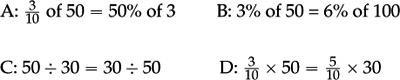
=  ”. Something similar arises in the algebra of expressions, where pupils first learn that, given a jumble of symbols on the left hand side, one is expected to simplify it in some way and set it “equal” to something a bit like an “answer” (on the right hand side). For example one might be given an expression such as
and be expected to rewrite it as “= x2 − x” (or as “= x(x – 1)”). However one later broadens this use of the equals sign so that “=” simply links two expressions that are “algebraically equivalent”—that is, where one side can be transformed into the other side via the rules of algebra. Any such equation that links two expressions that are algebraically equivalent is called an identity.
Pupils become aware of these four subdomains gradually, generally starting with formulae, then equations and expressions. The goal throughout should be to establish two main principles:
•letters are essentially placeholders for numbers, and so are subject only to the laws of arithmetic (or algebra);
•in formulae and equations, the letters can take any values that are consistent with the constraint expressed by the formula or equation; in an expression or identity the only constraints are the laws of arithmetic—so the x in “ ” cannot be set = 0, but otherwise the letters can be replaced by any values whatsoever, as long as different instances of the same letter are given the same value.
substitute values into expressions, rearrange and simplify expressions, and solve equations
2.1.3.1The requirement in 2.1.3 reinforces the immediately preceding bullet point. In an equation, the letters are constrained, so can only take particular (as yet unknown) values.
•In contrast, the letters in an algebraic expression are only required to satisfy the rules of arithmetic (or of algebra), so can be replaced by any numbers whatsoever (provided they are not clearly “forbidden values”—such as those that would make a denominator equal to zero).
Many pupils never grasp this fact, and so move letters around without realising that they are little more than placeholders for numbers, and must be treated as such. Pupils need more experience of substituting given numerical values for the letters in an expression, in order to internalise the idea that a letter can be given any value provided all occurrences of the same letter are given the same value. The act of substituting and evaluating also provides opportunities
•to exercise mental arithmetic, and
•to check that standard algebraic notation (juxtaposition as multiplication, brackets, powers, the fraction bar notation, priority of operations, etc.) is translated correctly when calculating with numbers.
Moreover, evaluating expressions in this way begins to convey the key idea that
•each choice of inputs gives rise to a single, determined output value for the expression.
That is, such expressions provide the simplest examples of what we will later call a function (of its component variables).
2.1.3.2The expression “rearrange and simplify” in the quote at the start of 2.1.3 gives a slightly misleading impression. Algebra almost never involves “rearranging” for the sake of it: one “rearranges” the terms of a compound expression for a reason—and that reason is almost always to simplify in some way. We are formally allowed to rearrange, or to manipulate, expressions in any way that respects the rules of algebra; but in practice we ignore almost all rearrangements, and focus on those which seem likely to lead to a more manageable, or “simpler”, result. Hence “rearrange and simplify” might have been better expressed as
“rearrange in order to simplify”.
In any event it is clear that pupils need more exercises (and class discussion) to help them learn what kinds of outputs are mathematically “simpler” (such as “fully cancelled” expressions, or those in “fully factorised” form), and to understand when and why the simpler forms are to be preferred.
2.1.3.3The requirement at the start of Subsection 2.1.3 ends with three innocent-looking words: “and solve equations”. In mathematics the expression “solve equations” strictly means “solve exactly”—by algebraic methods. We delay further comment on exactly what this means until Subsection 2.2.2.2. However, once this basic notion is understood, it can be modified, or re-interpreted in other fruitful ways.
The first such reinterpretation is to interpret the equations and the solving process geometrically. This reinterpretation does not help in the solution process itself, but it gives rise to interesting applications; it also provides a valuable alternative way of thinking about what is going on.
A different variation on the idea of “solving an equation” arises when we have no obvious way of finding an exact solution. It is then worth looking for effective ways of “getting close to” the elusive exact solution—that is, to find an approximate solution. The standard way to do this is to devise a process which allows us to “creep up on” a solution by generating a sequence which approaches the exact solution ever more closely. And the preferred kind of process is one which always takes the output from the previous step and operates on it in the same way to get the next approximation. This kind of repetition of a single process is called “iteration”—an idea which appears unannounced in the GCSE specification.10 There, in item 20 under the heading Number, we read:
find approximate solutions to equations numerically using iteration;
and in item 16 of Ratio, proportion, and rates of change we read:
work with general iterative processes.
There is no officially required preparatory work at Key Stage 3. However, when finding approximate points of intersection of two straight lines, or of the graph of a curve and the x-axis, it may make sense to alert pupils to the desirability of having a deterministic numerical (rather than graphical) process that finds such solutions to any required degree of accuracy. At the same time one can prepare the ground as part of work with sequences, by exploring the behaviour of standard sequences that “converge” (such as  , or
, or  , or
, or 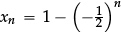 , or
, or  ), and others that “diverge” (such as xn = 10n, or xn = 2n).
The geometrical interpretation of the meaning of “solve” arises because algebraic equations correspond to geometrical curves or surfaces. This important link between algebra and geometry was forged by Descartes (1596-1650), who in 1637 showed that solving an equation corresponds to
•looking for points on a curve or surface where some expression takes a particular value (as with contour lines on an Ordinance Survey map); or
•looking for points where a curve or surface intersects a line (such as the x-axis), or a plane.
Hence the solutions of an equation, or of a system of equations, can be thought of as the coordinates of some point or points where two or more curves, or surfaces, meet. This is a powerful idea which can help to explain, for example,
•why some quadratic equations, such as x2 + 1 = 0, have no solutions (because the curve y = x2 + 1 never crosses the x-axis—that is, the line “y = 0”),
•why other quadratic equations, such as x2 = 0, have just one solution (because the curve y = x2 touches the x axis “y = 0”), and
•why many quadratic equations, such as x2 − 1 = 0, have exactly two solutions (because the curve y = x2 − 1 cuts the x-axis “y = 0” in two points: (−1,0) and (1,0)).
The geometrical interpretation makes it possible for pupils to engage the hand and the eye to draw the relevant curves and to find the approximate coordinates of the points which correspond to solutions of the given equation(s)—a process that can help the brain to make sense of the exact algebraic solution process, which might otherwise remain a purely abstract idea. Without the insights provided by this geometrical interpretation, pupils can all too easily misapply the rules of algebra—even with such simple examples as:
•x = x2 (where thoughtless cancellation can easily lead one to lose the solution x = 0). If we interpret solutions of this equation as the two points (0, 0) and (1, 1) where the familiar curves y = x and y = x2 cross, this can illustrate the error, can underline the importance of only cancelling factors which are never zero, and can help to reinforce the reasons for the standard algebraic method (when dealing with quadratics and higher powers) of
“taking everything to one side and factorising”.
The same idea applies to less familiar equations such as
•x = 2x4 (or x = 3x5) where one can again consider the two points where the curves y = x and y = 2x4 cross (or the three points where the curves y = x and y = 3x5 cross).
Later one can apply the same idea to cos x = 1, to sin x =  , or to x = tan x, to see that each equation has infinitely many solutions.
Sketching the lines or curves corresponding to two equations can allow one to find approximate solutions by estimating the coordinates of the points where the lines or curves intersect. This kind of geometrical visualisation is didactically and psychologically invaluable. But it is not a logical, or mathematical way of actually “solving the equation”—any more than the unknown length of the hypotenuse of a right angled triangle with legs of lengths 3 and 4 (or a and b) can be mathematically calculated by drawing an approximate 3 by 4 rectangle (or an a by b rectangle) and then measuring the diagonal.
2.2.1 [Reason mathematically p. 4]:
extend and formalise their knowledge of ratio and proportion
The words “ratio” and “proportion” are here used correctly! But they are so often used incorrectly that we go into considerable detail (here and in Part III, Section 1.9) to explain the background that is needed if pupils are to “formalise their knowledge of ratio and proportion”. We should perhaps stress that our comments throughout are designed to provide food-for-thought for teachers, and are not intended to constitute a teaching sequence for pupils.
Elementary mathematics comes into its own (and needs to be seriously taught!) as soon as we take the step from addition to multiplication. Ratios are the quintessential “multiplicative relations”, and work with ratios links naturally to work with fractions.
The basic “knowledge of ratio and proportion” which all pupils need to build on is relatively familiar and accessible to all: so all can make some progress. And this matters, because the topic is important, and has many applications. However, the step that leads from a “common sense” view to its mathematical analysis is more delicate; and though the art of teaching consists in finding ways to make such things easier to digest, one should not underestimate the challenge in this case.
The initial stage is purely numerical.
A position is advertised at £8.30 per hour (including specified breaks).
If my weekly schedule counts as 25 hours, then I expect to earn
25 × £8.30 = £207.50.
Here the given data includes the “unit cost” of “earnings per hour”, and the calculation reduces to a single multiplication. Despite the disturbingly low success rate for problem 1.4J above, this kind of multiplication can be made accessible to almost everyone. So it should be possible (even if it takes time and care) to extend this idea to problems where the “unit cost” has to be extracted first, before it can be used to find the required answer:
If my schedule counts as 25 hours per week and I earn £207.50, what would you expect to earn if your schedule counted as 30 hours?
All that is needed is to insert an extra reverse step, before repeating essentially the same calculation:
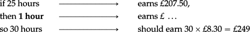
In other words, all that is needed (once one has a template to organise one’s thoughts and calculations) is to carry out two multiplications (“ ×  ” and “ ×30”) instead of one multiplication. This two-step process, where the unit cost is extracted first, is often referred to as “the unitary method”.
The general situation of which the above is an example arises whenever two quantities, in this case
“hours worked”and“pay received (in £)”
vary together in such a way that, whenever we have two linked pairs of quantities, such as:
25 hourscorresponds to£207.50,
and
30 hourscorresponds to£249,
then the ratio between the two quantities of the first kind
25 : 30
is equal to the ratio between the two quantities of the second kind
207.50 : 249
This “equality of ratios” is called a proportion. We also say “the two quantities—hours worked, and pay received—vary in proportion to each other”. (Slightly confusingly, this is sometimes referred to as “direct proportion”—to underline the contrast with “inverse proportion”, where the two quantities x, y vary in such a way that the first quantity x varies in proportion to the inverse  of the second quantity).
The “equality of ratios” can be re-written as an equality of fractions:

This is all very well, but each time we choose a different “linked pair of quantities” we get two new ratios. The new ratios are again equal, but they are different from the previous two ratios that were equal. However, if we rewrite the fraction equation in the form

then something remarkable happens: we obtain a quotient which is always the same—and which is called the constant of proportionality.
Teachers and schools will no doubt have their own ways of simplifying this idea. But there is no escaping from the need to prepare the ground by doing sufficient prior work with word problems, with multiplication and division, with fractions, and with ratios.
The teacher is like a midwife—using their own higher knowledge to coax ideas into pupils’ minds. But to do this effectively, the teacher (like the midwife) needs to see the bigger picture—even if they then choose to suppress some of the details. To generate a ratio, all that is needed is a single class of pairwise comparable magnitudes (that is, a class of magnitudes where any two given entities can be ‘compared’, so that we can decide which is the larger). The simplest examples of such a class of “comparable magnitudes” are the set of positive rational numbers, and the set of positive real numbers. In the context of ratios, real numbers generally arise as the set of possible numerical measures of some set of objects (relative to some chosen unit). Numerical ratios are easier to handle (replacing the class of objects by their measures). But ratios are not necessarily numerical. They arise naturally in mathematics whenever one has a class of “comparable entities” (such as line segments, or 2D shapes): we do not have to turn everything into numbers by measuring (for a very simple example, see Part III, Section 1.9.2).
The example above illustrates how a proportion arises whenever two different classes of entities are linked in a special (but very common) way. For example, suppose that one class consists of
“quantities of petrol”
and the other class consists of
| “amounts of money in £”. |
If 1 litre of petrol | costs £1.50, |
then we expect 2 litres | to cost £3 (= 2 × £1.50) |
That is, for any two purchases from the same outlet at the same time,
the quantities purchased (in litres)
are in the same ratio as
| the amounts paid (in £). |
If I buy a litres of petrol | and pay £c, |
and you buy b litres of petrol | and pay £d, |
then the ratio a : b | is equal to the ratio c : d. |
The equality
a : b = c : d
is what we call a proportion.
Note that since a, b, c, d are magnitudes, with a, b of one kind and c, d of another kind, then a : b is a perfectly well-defined ratio; but “a : c” makes no sense, because a and c are not comparable magnitudes. One cannot have a ratio between a quantity of fluid and an amount of money. However, if we replace the different quantities and amounts by their numerical measures, then the equality of ratios “a : b = c : d” can be written as an equation between fractions, which can then be treated purely numerically (or algebraically), to give an equality of quotients, or fractions:
| (*) |

The two quotients in equation (*) are always equal, but can take any positive value. You could consider buying
b = 2a litres of petrol | and pay d = 2c pounds, |
and the quotients would then both take the value  . Or you could buy
| and pay |
 litres of petrol
 pounds,
and the quotients would then both take the value 2.
However, if we now treat the equation (*) purely algebraically, then we can rewrite it in the form

This equation looks very similar to equation (*), but it is completely different. The two sides do not represent ratios, but specify the constant of proportionality (relative to the two chosen units: litres and pounds (£)). That is, once we choose units and give numerical values a and c to the basic pair of corresponding magnitudes—one from one class and one from the other
a litres ![]() cost £c
cost £c
the value of the quotient  is a constant, the constant of proportionality. That is, it has the same value as the corresponding quotient
  for any other pair of corresponding magnitudes b, d (one from one class and one from the other).
This is the simplest, and perhaps the most valuable, application of school mathematics—to life, to science and to mathematics itself. It applies whenever two quantities are related so that if one quantity doubles, or triples, so does the other: that is, where the numerical measures a, c or b, d of the two quantities have a constant ratio. Two quantities that vary in such a way as to preserve a constant ratio between their values are said to be “in proportion”.
The fact that “ is a constant” means that the number lines corresponding to the two families of measures “line up” in such a way that one scale is simply a multiple
  of the other:
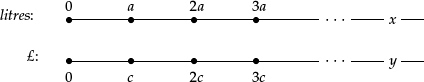
If we imagine a linked pair (x, y) of unknown variables—where “x litres costs £y”—then these variables are connected by the linear equation

Any particular proportion problem that pupils may be required to solve is likely to involve just two pairs (a, c) and (b, d),
•where a and b come from one class of magnitudes, and c and d come from the other class.
In a typical proportion problem, three of the four values are given and the fourth is to be found. Hence one pair is completely known, and we take this as our “base”, or “reference pair”:
a litres ![]() cost £c
cost £c
One of the other two values b, d is “to be found”. So the four ingredients can be thought of as the corners of a rectangular array, where three of the values are known and the fourth is to be calculated:
Ifa litres ![]() cost £c
cost £c
then b litres ![]() cost £??
cost £??
Alternatively, the missing value may be the one in the bottom left corner:
Ifa litres ![]() cost £c
cost £c
then ?? litres ![]() cost £d
cost £d
This standard way of representing the four pieces of information in a proportion—with three known values and one generally unknown—is referred to here as the rectangular template for displaying proportion problems. We will revise and extend this example in Part III (p. 137ff).
2.2.2 [Reason mathematically p. 4]:
–make and test conjectures about patterns and relationships; look for proofs or counterexamples
–begin to reason deductively in geometry, number and algebra, including using geometrical constructions
Learning to distinguish between a plausible guess and a provable fact should be part of school mathematics from the earliest years. In Key Stage 3 this distinction takes on a new importance—but the requirement stated in 2.2.2 is difficult to interpret because the logical framework within which such deduction is to take place remains undeclared (e.g. for Euclidean geometry).
2.2.2.1The problems begin already with the requirement to “reason deductively in number” when making sense of simple numerical patterns. At present the patterns pupils meet are often chosen in a way that misleads everyone into thinking that
patterns that seem genuine, always are genuine.
This makes it hard for pupils to discover the need for proof.
Consider, for example, the first 17 terms of what should be a familiar endless sequence:
2, 4, 8, 16, 32, 64, 128, 256, 512, 1024, 2048, 4096, 8192, 16384, 32768, 65536, 131072, …
These are the successive powers of 2. Pupils can extend the sequence as far as they need simply by repeatedly multiplying by 2.
Now consider the two sequences that arise naturally from this sequence of “powers of 2” by looking at the two “ends” of each term of this sequence:
first the succession of units digits:
2, 4, 8, 6,2, 4, 8, 6,2, 4, 8, 6,2, 4, 6, 8,2, …
then the succession of leading digits:
2, 4, 8, 1, 3, 6, 1, 2, 5, 1,2, 4, 8, 1, 3, 6, 1, 2, … .
As one continues to extend the original sequence of powers of 2, it is hard not to notice that both these sequences of digits seem to recur.
But do they really? And if they do, are these two conjectures really similar?
It is relatively easy to prove that the first sequence “2, 4, 8, 6, 2, 4, 8, 6, …” really does recur. For we know that when we carry out the short multiplication, multiplying by 2 each time,
•each new units digit arises from multiplying the previous units digit by 2.
So each time we reach a units digit of 2, we notice that
–the units digit of the next term is 4 (since “2 × 2 ends in 4”);
–then “2 × 4 ends in 8”;
–then “2 × 8 ends in 6”;
–then “2 × 6 ends in 2”—and the sequence “2, 4, 8, 6” starts to repeat.
However, the second sequence
2, 4, 8, 1, 3, 6, 1, 2, 5, 1,2, 4, 8, 1, …
is different. There is no obvious reason why the leading digits should recur as they seem to do.
Somehow pupils need to learn that what looks like a pattern may not be a pattern at all!
So we have to insist that, in the absence of an acceptable proof, no pattern is simply “believed”—no matter how persistent it may seem to be.
2.2.2.2The requirement to “reason deductively in algebra” is more interesting—and is explored surprisingly rarely. Proof in algebra has to be based on combining
•use of the commutative and associative laws of addition and multiplication, and the distributive law, to simplify expressions,
together with
•the idea that one is allowed to operate on the two sides of any equals sign in the same way without destroying the equality.
The most obvious example at Key Stage 3 and Key Stage 4 (about which the programme of study remains stubbornly silent) is the proof that
(−1) × (−1) = 1.
There are all sorts of heuristic arguments that can be used to “justify” this crucial mathematical fact. One of the more plausible explanations is to consider dieting and weight loss.
•If I consistently put on 1kg per month, then
in 3 months time, I will be (3 × 1)kg heavier than now; and
3 months ago, i.e. “in −3 months time”, my weight was [(−3) × 1]kg more than now.
•If I consistently lose 1 kg per month (that is, if I “put on (−1)kg per month”), then I know that
in 3 months time, my weight will be 3kg less than it is now; and
(*) 3 months ago, my weight would have been 3kg more than it is now.
If we try to express these observations arithmetically we see that
in 3 months time, my weight will be [3 × (−1)]kg more than it is now; whereas
(**) 3 months ago, my weight must have been [(−3) × (−1)]kg more than it is now.
Taken together (*) and (**) seem to suggest that: (−3) × (−1) = 3.
Such linguistic plausibility is fine at Key Stage 3. But at some stage in Key Stage 4, those who may move on to A level need to know that the fact has a simple mathematical basis. All we need to use is that:
(i) | multiplying by 1 changes nothing: a × 1 = a for all a; |
(ii) | adding 0 changes nothing: a + 0 = a for all a; |
(iii) | the distributive law holds. |
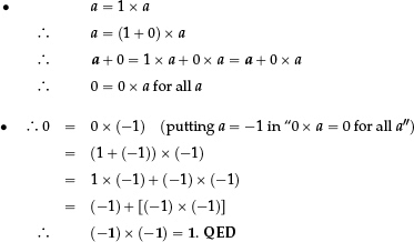
The proof given here is for teachers, and is based on the fact that
(i) | is the defining property of the multiplicative unit “1”, and |
(ii) | is the corresponding defining property of the additive identity “0”. |
Some readers may judge that for pupils the initial step—the fact that “0 × a = 0 for all a”—is so familiar that the first bullet point is best suppressed.
A quite different fact that is often confused with the above is the fact that “subtracting a negative is the same as adding”:
a − (− x) = a + x.
However tempting it may seem, little is gained by summarising this and the result proved above as “two minuses make a plus”. The two results are in fact rather different: in the above equation there is no multiplication in sight. Moreover, the symbol “−x” should not be referred to as “a negative”, since its value depends on the value of x itself: it is simply the “additive inverse of x”; that is, “−x” is the “negative of x”, or that number which cancels out “x” under addition and produces 0.
Claim a − (−x) = a + x for all a, x
(i) | a + (−x) + x = a + 0 = a |
∴ a + (−x) = a − x
(ii) | a − (−x) + (−x) = a |
∴ a − (−x) − x = a
Now add x to both sides:
∴ a − (−x) = a + x.QED
At Key Stage 3 schools will need to develop their own ways of achieving fluency in using such algebraic rules—for they are far from obvious! If the proof is illustrated numerically, one must first establish part (i), so that it can be used in part (ii); and it is important to give three or four examples—e.g. replacing a and x first by 1 and 2, then by 1 and −2, then by −1 and 2, and finally by −1 and −2.
A rather different opportunity for pupils to “reason deductively in algebra” arises in the solution of equations. We pointed out in Subsection 2.1.3 that “to solve equations” really means to solve exactly—by algebraic methods. A given equation in a single unknown “x” has an imagined (but unknown) set of “solutions”, or possible values for the unknown “x”. The art of solving equations algebraically is a process which exploits exactly two kinds of moves.
•The first kind of move allows us to replace any constituent expression on either side of the equation by another expression which is algebraically equivalent to it. Because “algebraically equivalent” expressions are equal for all values of x, this kind of move is reversible, so exactly the same values of the unknown “x” satisfy the new equation as satisfied the old equation.
•The second kind of move is to subject both sides of the equation to the same operation.
–If this operation is reversible (such as adding or subtracting the same thing from both sides, or multiplying or dividing both sides by a given expression that is never equal to zero, or cubing both sides), then we can again be sure that exactly the same values of the unknown “x” satisfy the new equation as satisfied the old equation.
–However, we are also free to subject both sides of the equation to an operation which is not reversible, such as squaring both sides of the equation. In this case we can only be sure that
any value of “x” which satisfied the original equation will also satisfy the new equation.
That is, any solution of the original equation is also a solution of the new equation, so we can be sure that we have not lost any solutions. However, we may have gained some new solutions which did not satisfy the original equation. For example,
if “A = B”, then we can square both sides to get the new equation “A2 = B2”;
but the change may introduce new solutions, since A2 = B2 includes the possibility that A = −B, which is quite different from the original equation.
A third domain where pupils should learn to “reason deductively in algebra” arises with inequalities. In many ways equations are rather rare. In mathematics and in life inequalities are much more common. For example, a business never quite ‘breaks even’: it either makes a surplus, or it makes a loss. And for a production line to keep running, one can never order the exact amount of material that is required: one has to slightly over-order to make sure that the supply of what is needed never runs out (and one would like to do so in such a way that waste is reduced to a minimum). This means that real problems are often formulated in terms of inequalities.
Much of what holds for equations translates to inequalities.
•The solution of a linear equation in one unknown “x” is a single point on the x-axis; and the solution of the corresponding linear inequality consists of all values on one side of this point (a “half-line”).
•The possible solutions of a linear equation in two variables x, y correspond to the set of all points (x, y) on a line, which divides the plane into two “half-planes”; and the solutions of the corresponding linear inequality in two variables x, y consists of all points on one side of the line—that is, in one of the two half-planes.
The algebraic rules for “solving inequalities” are very similar to the rules for solving equations. For example, one is allowed to add the same to both sides of an inequality, or to multiply both sides of a given inequality by a positive quantity. But there is a twist: a negative multiplier reverses the inequality!
The extent to which inequalities are neglected in England is clear from one of the 2011 TIMSS Year 9 items:
2.2.2.2A“Solve the inequality: 9x – 6 < 4x + 4”.
We can transform the given inequality by collecting terms (or more correctly, by “adding 6−4x to both sides”) to get 5x < 10.
We can then multiply both sides by the positive multiplier  to obtain “x < 2”.
The percentage of correct responses to this problem from a representative sample of 15 year olds in more than 50 countries was not encouraging, and included:11
2.2.2.2AKorea 60%Russia 46%Hungary 38%USA 21%Australia 8%England 3%
This suggests rather starkly that our approach to deduction and calculation in algebra needs to change in order to establish a clear connection between the familiar processes used in solving equations and those required to solve inequalities (which are listed in the Key Stage 3 programme in the third bullet point of “Algebra”, and which feature in the GCSE mathematics subject content list, so certainly warrant preliminary work at this level—even if a more formal treatment can be delayed until Key Stage 4).
2.2.2.3The requirement to “begin to reason deductively in geometry” and to include “geometrical constructions” is in some ways easier to achieve. But it is in other ways more delicate.
Geometry at Key Stage 1 and 2 is predominantly experiential and descriptive. However, once the basic repertoire of shapes and language has been established, one can begin to organise the subject matter at Key Stage 3 into a logical, or deductive, hierarchy. For example:
•once one knows that angles at a point P on a straight line add to 180°,
•one can prove that, whenever two lines cross at a point P, any pair of vertically opposite angles A and A′ at P are necessarily equal:
[Proof: Let B be the angle “between” the two vertically opposite angles A and A′. Then A + B is the straight angle on one line, and B + A′ is the straight angle on the other line.
∴ A + B = B + A′, so A = A′. QED]
This proof only depends on the assumption (which pupils and teachers alike accept without even noticing) that:
all ‘straight angles’ (at possibly different points on two straight lines) are equal.
Plane geometry deals with imagined points and lines. Two points determine exactly one line, and two lines which are not parallel meet in exactly one point. This much should be clear—though it needs to be reinforced in Year 7 through appropriate drawing exercises.
More importantly, the methods and language of geometry require us to make a clear distinction between
•the line AB (which passes through the two points A, B, and which extends forever in both directions)
and
•the line segment AB (that starts at A, runs to B, and then stops), which in the UK is usually also written as AB.
For example, the sides of triangle ABC are not the “lines” AB, BC, CA, but rather the line segments AB, BC, CA. Geometrical experience prior to Year 8 needs to ensure that these ideas can be taken for granted without drawing explicit attention to them. However, to go further, one needs a clear framework within which the basic results of Euclidean geometry can be derived. And since such a framework remains largely implicit (or even hidden) in the programme of study, it may help if we give (here and in Part III, Section 3) a brief outline of the necessary background.
The whole of geometry in 2D and in 3D rests on one key idea, which needs to be cultivated at Key Stage 2, and strengthened at Key Stage 3 through drawing, and through making and examining standard structures. This is the discovery that triangles hold the key to the construction and analysis of more complicated shapes. Every integer can be factorised as a product of prime numbers, and this factorisation tells us important things about the original number, even though most of the details of this factorisation cannot be seen when one first looks at the starting number. In much the same way important properties of complicated geometrical configurations can be analysed in terms of their constituent triangles, even though these triangles may not be immediately apparent in the initial configuration. (This strategy of reducing geometrical reasoning in general to reasoning about triangles is also related to the fact that the rigidity of structures in engineering—such as cranes, or roof trusses, or bridges, or the Wembley arch—often comes down to the way triangles are built in to their design.)
Mathematics succeeds by translating sense impressions and language, or sounds, into symbols which allow exact calculation. “The sum of three consecutive even integers” makes perfect sense in English, but the words alone suggest nothing special. However, as soon as we translate the words into symbols and write this as
2n + (2n + 2) + (2n + 4) = 6n + 6
it is clear that the result is always a multiple of 6. The same is true in geometry. The English words “triangle” or “quadrilateral” may conjure up a visual impression in the mind’s eye of an imagined shape. But one cannot calculate with such an impression. If we wish to refer to a particular triangle or quadrilateral, we may point it out; and others may notice things about the indicated shape; but they cannot talk, or reason deductively about a triangle or quadrilateral which has been indicated in this way. Just as “consecutive even integers” were given names in accordance with the rules of algebra, so a triangle or quadrilateral has to be given a name in accordance with certain conventions before we can begin to calculate with it.
Labelling conventions have to communicate reliably between individuals, and so are chosen to reflect the underlying geometric structure. For example, a polygon is a collection of line segments, where successive pairs meet at a shared vertex. Hence the sequence in which the vertices are labelled matters. A quadrilateral ABCD has to be labelled in cyclic order, where the edges are the successive line segments, or edges, that make up the quadrilateral: AB and BC (meeting at B), BC and CD (meeting at C), CD and DA (meeting at D), and DA and AB (meeting at A). Just as the neglect of grammar and spelling makes it impossible for pupils to organise and to express their thoughts, and hence to be understood, so it is an indication of the anarchy in English school geometry that standard geometric conventions are routinely flouted without the serious consequences being recognised.
There is another oversight which may prove harder for some to swallow. The reader is invited to imagine (and to draw, and to label) two adjacent unit squares—ABCF, FCDE. The squares ABCF and FCDE are clearly different, but very much alike. But we would not usually quibble if I referred to the first square as ABCF and you referred to it as BCFA (or even BAFC—but not AFBC). However, ABCF and BCFA are in some sense different—whether they are different squares or just different labellings need not be decided immediately. The difficulty may be clearer if one considers the two rectangles ABDE and DBAE: much of the time one may loosely think of these as “different ways of referring to the same rectangle”. But life is much easier if one views them as different—though closely related. This becomes clear as soon as one tries to sharpen the feeling that the two rectangles are “the same”, or “congruent”; for then the “sameness” one is trying to capture requires one to match them up in a way that essentially changes the labelling of the second rectangle, since “AB” (the first side mentioned in ABDE) is a short side, whereas “DB” (the first side mentioned in DBAE) is a long side. It does not matter whether the matching up leads one to think of the second rectangle as ABDE, or BAED, or DEAB, or EDBA; but it becomes silly to insist on calling it DBAE while also insisting that it is “the same as ABDE”. Even if we do not strictly insist on such precision all the time, each time we do some kind of “calculation” with a triangle, or a quadrilateral, we find that the order matters (as well as the sequential labelling of the vertices).
So there is a clear sense in which, whenever push comes to shove, a “triangle” is not just a three-cornered shape: it is a labelled, or ordered, triple ABC, where the order matters. (If one only knows the three vertices, but not the order, then this corresponds to several different triangles: ΔABC, ΔBCA, ΔCAB, ΔBAC, … .)
Each triangle involves six different pieces of data:
•the three side lengths: AB = c, BC = a, CA = b, and
•the three angles: ∠ABC (often abbreviated as “B”), ∠BCA (abbreviated as “C”), and ∠CAB (abbreviated as “A”).
There are three basic organising principles on which deductive reasoning in geometry is based. Two of these principles (relating to congruence and to parallels) belong naturally to Key Stage 3; the third organising principle (the similarity criterion) belongs slightly later—perhaps in Year 9 or Year 10.
The first organising principle is the congruence criterion. This underlines the central role played by triangles, and should arise naturally as a formal summary of pupils’ extensive experience from drawing, where they should discover that:
one does not need to know everything about a triangle in order to specify it uniquely.
The “congruence criterion” then summarises the information that is needed to specify a triangle uniquely.
Two (ordered) triangles ΔABC and ΔDEF are congruent if the (ordered) correspondence

matches up each of the six ingredients of triangle ΔABC with those of triangle ΔDEF in such a way that
•all three corresponding pairs of line segments are equal: AB = DE, BC = EF, CA = FD, and
•all three corresponding pairs of angles are equal: A = D, B = E, C = F.
We write this as: ΔABC ≡ ΔDEF (which we read as “Triangle ABC is congruent to triangle DEF”).
“Congruence of triangles” only makes sense between ordered triangles. And it can help pupils to see more clearly which vertex of the first triangle corresponds to which in the second triangle, and which side of the first triangle corresponds to which in the second triangle, if pupils initially write:

since this lines up
•corresponding vertices (with A directly above D, B directly above E, C directly above F), and
•corresponding sides (with AB directly above DE, BC directly above EF, CA directly above FD).
Pupils’ experience of drawing should then reveal that, in order to guarantee congruence
“just three pieces of data suffice”,
provided we avoid the two triples that don’t suffice! Hence they need to understand
•that any of SSS, SAS, ASA determine the triangle uniquely,
•that “AAA” determines the shape, but says nothing about the scale, or size, of the triangle;
•that the appropriately named “ASS” criterion is different, in that it may give rise to two possible triangles (for example, a triangle with ∠B = 30° and BC =  , CA = 1 could have either AB = 2 with ∠A acute, or AB = 1 with ∠A obtuse).
The congruence criterion summarises the first of these three bullet points:
•triangles ΔABC and ΔDEF are congruent (by SSS) if AB = DE, BC = EF, and CA = FD;
•triangles ΔABC and ΔDEF are congruent (by SAS) if AB = DE, ∠BAC = ∠EDF, and AC = DF;
•triangles ΔABC and ΔDEF are congruent (by ASA) if ∠BAC = ∠EDF, AB = DE, and ∠ABC = ∠DEF.
The RHS congruence criterion is not part of this basic congruence criterion, so does not really belong at this stage. It arises as the degenerate instance of the failed ASS criterion (where the angle “A” in “ASS” is a right angle, and so is neither acute nor obtuse). The fact that RHS guarantees congruence follows somewhat later (once we have proved Pythagoras’ Theorem, since knowing two sides and a right angle then determines the third side. So RHS is a special case of SSS).
SSS, SAS, and ASA congruence allow one to prove such results as:
•The two diagonals of a square ABCD are equal
[Proof The two triangles ΔABC, and ΔBCD are congruent by SAS:
ΔABC
≡ ΔBCD(since AB = BC, ∠B = ∠C, and BC = CD).
Hence AC (in ΔABC) = BD (in ΔBCD). QED].
•The base angles of an isosceles triangle are equal:
[Proof 1 Suppose AB = AC. Construct the midpoint M of the base BC. Then, by SSS,
≡ ΔAMC(since AM = AM, MB = MC (M is the midpoint of BC), and AB = AC (given)).
Hence ∠ABM (in ΔAMB) = ∠ACM (in ΔAMC). QED].
It is worth pondering on a different proof of this result, which exploits the fact that ΔABC and ΔACB are different triangles.
[Proof 2 Suppose AB = AC. Then the two different ordered triangles ΔBAC, and ΔCAB are congruent by SAS:
ΔBAC
≡ ΔCAB(since BA = CA, ∠A = ∠A, and AC = AB).
Hence ∠B (in ΔBAC) = ∠C (in ΔCAB). QED].
•Any triangle with equal base angles is isosceles:
[Proof Suppose ∠ABC = ∠ACB. Then the two different ordered triangles ΔABC, and ΔACB are congruent by ASA:
ΔABC
≡ ΔACB(since ∠ABC = ∠ACB, BC = CB, and ∠BCA = ∠CBA).
Hence AB (in ΔABC) = AC (in ΔACB). QED].
•In an isosceles triangle, the bisector of the apex angle, the median to the base, and the perpendicular to the base are all the same.
Isosceles triangles constitute one of the simplest and most fruitful sources of geometrical deduction. For example, in a circle any chord AB forms an isosceles triangle OAB with the centre O, so isosceles triangles allow one to deduce all sorts of properties of circles (the so-called “circle theorems”).
The congruence criterion is also needed to prove that the basic ruler and compass constructions do what they claim to do:
•to bisect a given angle,
•to bisect a given line segment,
•to construct a perpendicular to a given line from a given point, and
•to construct a line parallel to a given line through a given point.
For example:
•To bisect a given angle ∠BAC. Let the circle with centre A and passing through B meet the half line AC at the point B′. Let the two circles—one with centre B and passing through A, the other with centre B′ and passing through A— meet again at D. Then AD bisects ∠BAC.
[Proof We show that ΔBAD ≡ ΔB′AD (by the SSS congruence criterion), since
BA = B′A (both are radii of the same circle with centre A).
AD (in ΔADB) = AD (in ΔADB′) (the one segment is part of both triangles)
DB = AB (both are radii of the same circle with centre B)
AB = AB′ (both are radii of the same circle with centre A)
AB′ = DB′ (both are radii of the same circle with centre B′)
∴ DB = DB′.
Hence ∠DAB (in ΔBAD) = ∠DAB′ (in ΔB′AD), so DA bisects ∠BAC. QED]
The second organising principle in geometry is the criterion for two lines in the plane to be parallel.
Given any two lines in the plane, a transversal is a third line that cuts both of the two given lines. The parallel criterion declares that:
•two lines are parallel precisely when the alternate angles (or the corresponding angles) created by a transversal are equal.
This is a rather subtle criterion, but one which can be made thoroughly plausible. It immediately allows one to prove:
Claim The angles in any triangle ΔABC add to 180° (i.e. a “straight angle”).
Proof Construct the line XAY through vertex A which is parallel to BC (where X, B both lie on the same side of the line AC).
∴ ∠XAB = ∠CBA = ∠B (alternate angles)
and ∠YAC = ∠BCA = ∠C (alternate angles)
∴ ∠A + ∠B + ∠C | = ∠A + ∠XAB + ∠YAC |
| = ∠XAY (a straight angle at A on the line XY). QED |
And this in turn provides access to hundreds of wonderful (non-obvious, multi-step) problems involving angle chasing. This term is a shorthand for any activity in which a 2D configuration is specified, with the sizes of certain angles given, from which the sizes of other angles are to be logically determined (by reasoning and calculation, not by measuring). If the required angle were the third angle in a triangle whose other two angles were given, then the required angle could be immediately deduced. In general the size of the required angles may not be immediately deducible, but may force one to first calculate certain intermediate results. That is, angle-chasing refers to a restricted (geometrical) class of problems that are multi-step, and that are also deductive exercises in using the basic angle properties (angles at a point, angles on a straight line, vertically opposite angles, angles in a triangle—and later alternate angles). See for example, Extension mathematics Book Alpha by Tony Gardiner (Oxford 2007), Sections T9 and E2, and Book Beta Sections T17, C11 and E4.
If we combine the parallel criterion with the congruence criterion, we can prove the basic facts about parallelograms, and derive the fundamental fact that the area of a triangle is equal to
This then allows us to prove Pythagoras’ Theorem.
The congruence criterion and the parallel criterion allow one to transfer exact relations (such as equality of line segments or of angles) from one place to another. The third organising principle of secondary school Euclidean geometry, the similarity criterion, goes beyond this world of exact equality to allow one to deal with ratios, scaling, and enlargement. The introduction of this criterion is probably best delayed until the basic consequences of congruence and parallelism have been fully explored, and until pupils are sufficiently confident in working with ratio.
As with congruence, similarity in general is formulated in terms of “similarity of triangles”. The similarity criterion summarises the minimum requirement for two given triangles to be “similar”. Two (ordered) triangles ΔABC and ΔDEF are similar (which we write as ΔABC ~ ΔDEF) if
•corresponding angles are equal:
∠A = ∠D,∠B = ∠E,∠C = ∠F,
and
•corresponding sides are proportional:
AB : DE = BC : EF = CA : FD.
The similarity criterion may be thought of as a substitute for the (evidently false) “AAA congruence criterion”, in that it states that each of the above bullet points implies the other:
if corresponding angles are equal:
∠A = ∠D,∠B = ∠E,∠C = ∠F,
then corresponding sides are proportional:
AB : DE = BC : EF = CA : FD;
and
if corresponding sides are proportional:
AB : DE = BC : EF = CA : FD,
then corresponding angles are equal:
∠A = ∠D,∠B = ∠E,∠C = ∠F.
Special cases of this can be proved using the exact relation of congruence. For example, one can prove the Midpoint Theorem, which says that:
if in ΔABC, M is the midpoint of AB and N is the midpoint of AC,
then MN is parallel to BC and BC : MN = 2 : 1.
That is ΔABC ~ ΔAMN, with the corresponding scale factor AB : AM = AC : AN = BC : MN = 2 : 1.
Some further detail concerning geometry may be found in Part III, Section 3.
2.2.2.4The requirements listed at the start of Section 2.2.2 suggest that during Key Stage 3 pupils should
“make and test conjectures”
and
“begin to reason deductively”.
This should be interpreted as part of the (unstated) requirement that pupils should at all times expect the methods of elementary mathematics to make sense. But there are different kinds of “sense making”: some involve inference; some involve plausibility arguments; and some are rooted in deduction. The requirement for pupils to “reason deductively” means that they need to be clear
•when they are experimenting or conjecturing, and when they are working “deductively”;
and also
•when they are working in rough, and when they are writing for others to read.
That is, they need some way of demonstrating (to themselves and to others) which mode they are in at any given time. For pupils who are ready for the formal procedures of elementary mathematics at Key Stage 3, the calculations and methods should be increasingly justified in ways that are exact and deductive (rather than approximate, inferential, or based on the authority of the teacher). The essence of elementary mathematics at secondary level incorporates the twin facts
•that its domain is restricted and abstract, and
•that within this limited domain, the knowledge it delivers is certain—that is, objective, rather than subjective (or approximate, or based only on experience, or conjecture, or convention).
For such pupils calculations and solutions need to be increasingly presented in a way that constitutes a proof that the answer to the original problem is undeniably what emerges at the end of the calculation or solution. And this is best conveyed by laying out calculations and deductions line-by-line,
•with the given information, and any symbols representing “unknowns” declared at the outset,
•with each fresh step on a new line (and any explanation given alongside),
and
•with the final answer clearly displayed at the end.
The sequence of successive steps can then be grasped as a single chain of reasoning, in which each step follows clearly from those which went before. This logical structure is equally applicable
•to simple calculations,
•to the solution of an angle-chasing problem,
•to setting up and solving an equation,
•to proving that two algebraic (or trigonometric) expressions are identical,
•to a ruler and compass construction,
•to a proof (such as, that the angle in a semicircle is a right angle), or
•to the way pupils present their solutions to set problems.
It is hard to convey this style consistently in a discursive text such as this one. But it can be seen in the way we present short proofs. And it is also visible elsewhere—such as in the solution at the end of Section 2.3.5 below.
[Solve problems p. 5]:
–develop their mathematical knowledge, in part through solving problems and evaluating their outcomes, including multi-step problems
–develop their use of formal mathematical knowledge to interpret and solve problems, including in financial mathematics
–begin to model situations mathematically and express the results using a range of formal mathematical representations
–select appropriate concepts, methods and techniques to apply to unfamiliar and non-routine problems
These four bullet points are clearly meant to encourage pupils and teachers to see school mathematics as more than endless practise with dry-as-dust formal technique. But beyond this admirable aspiration, it is far from clear what exactly is being advocated. We base our commentary on three questions.
•What is meant by a “problem”, rather than (say) an “exercise”?
•What does it mean to “solve problems”?
•And why are “multi-step” problems important?
2.3.1We begin by clarifying the distinction between “exercises” and “problems”.
An exercise is a task, or a collection of tasks that provide routine practice in some technique or combination of techniques. The techniques being exercised will have been explicitly taught, so the meaning of each task should be clear. Each sequence of exercises is designed to cultivate fluency in using the relevant techniques, and all that is required of pupils is that they implement the procedures more-or-less as they were taught in order to produce an answer. The overall goal of such a sequence of exercises is merely to establish mastery of the relevant technique in a suitably robust form. In particular, a well-designed set of exercises should help to avoid, or to eliminate, standard misconceptions and errors.
Exercises are not meant to be particularly exciting, or especially stimulating. But they can give pupils a quiet sense of satisfaction. Without a regular diet of suitable exercises, ranging from the simple to the suitably complex (including standard variations), pupils are likely to lack the repertoire of basic techniques they need in order to make sense of mildly more challenging tasks (as the examples 1.4A-1.4K above show). In other words,
exercises are the bread-and-potatoes of the mathematics curriculum.
Pupils in England clearly need more (carefully prepared) “bread-and-potatoes” exercises than they currently get. However, bread and potatoes alone do not constitute a healthy diet. Pupils also need more challenging activities both to whet their mathematical appetites, and to cultivate an inner willingness to tackle, and to persist with, simple but unfamiliar (or “non-routine”) problems. A problem is any task which we do not immediately recognise as being of a familiar type, and for which we therefore know no standard solution method. Hence, when faced with a problem, we may at first have no clear idea how to begin.
The first point to recognise is that a task does not have to be all that unfamiliar before it becomes a problem rather than an exercise! In the absence of an explicit problem solving culture, an exercise may appear to the pupil to be a problem simply because its solution method has not been mentioned for a week or so, or because it is worded in a way which fails to announce its connection with recent work. The second point is that the distinction between a problem and an exercise is not quite as clear-cut as we have made it look, and is to some extent time- and pupil-dependent. For example, an “I’m thinking of a number” problem from Year 5 or Year 6 should by Year 8 be seen to be a mere exercise in setting up and solving a simple equation.
Most useful techniques involve a chain of simple steps, and the technique as a whole is only an effective tool if the complete chain can be carried out entirely reliably—a requirement which may only be achieved after extensive practice. Examples include: any of the standard written algorithms; the process of turning a fraction into a decimal; the sequence of steps required to add or subtract two fractions, or to solve an equation or inequality, or to multiply out and simplify an algebraic expression. Hence each set of exercises should include tasks that force pupils to think a little more flexibly, and that require them to string simple steps together in a reliable way. Too many sets of exercises get stuck at the level of “one piece jigsaws”—with one-step routines being practised in isolation, ignoring key variations. Pupils need to learn from their everyday experience that the whole purpose of achieving fluency in routine bread-and-potatoes exercises is for them to learn to marshal these techniques to solve more demanding multi-step exercises, and more interesting, if mildly unsettling, problems.
2.3.2This distinction between exercises and problems affects how we choose to introduce each new topic or technique. Should we concentrate on relatively simple examples that minimise pupil difficulties, and which seem likely to guarantee a quick pay-off? Or should we—when working with the whole class—move quickly on to examples that provide a significant challenge, and so require pupils from the outset to grapple with (carefully chosen) tasks of a more demanding nature?
How challenging one can safely be will depend on the pupils. But experience from those who observe lessons in other countries suggests that the English preference for concentrating the initial worked examples on easy cases increases the extent of subsequent failure. Easy initial examples lead to cheap apparent success; but this initial pupil success may be based on pupils’ own inferred methods that appear to work in easy cases, but which are flawed in some way; or on backward-looking methods, that seem (to the pupil) to work in simple instances, but which do not extend to the general case. So we need to consider the benefits of starting each new topic with a harder “class problem” that brings out the full complexity of the method that we want pupils to master, and then to follow this up with exercises that may start simply, but which oblige pupils to think flexibly from the outset, and to handle standard variations including inverse problems.
2.3.3The last 30 years have witnessed a consistent concern about pupils’ ability to “use” the elementary mathematics they are supposed to know. Previous versions of the mathematics National Curriculum displayed an admirable determination to incorporate “Using and applying” within teaching and assessment. But such determination is not enough. The experience of the last 25 years in England is more useful as a guide to what does not work than to what does work. Much effort has been expended in trying to do better—but with limited effect. In particular, ambitious attempts to coerce change—using extended investigations, coursework, and “modelling”—have mostly served to demonstrate what should not be officially required at this level.
Somewhere along the line we seem to have lost sight of simple word problems. Word problems typically consist of two or three short sentences, from which pupils are required
•to extract the intended meaning and any required information,
•to identify what needs to be done,
and then
•to carry it out, and interpret the answer in the context of the problem.
Everyday uses of elementary mathematics tend to come in some variation of this form. Yet the simplest exercises, which might be solved routinely if they were presented without words, become powerful discriminators when given this gentle packaging. The need for pupils to read and extract the relevant data from two or three English sentences may appear routine—but it is a skill that has to be learned the hard way, and that constitutes the initial stepping-stone en route to the ultimate solution of almost any problem. This simple format can be tweaked to cover the standard variations of the underlying task (e.g. so that it appears both in direct and in the various indirect forms).
During Key Stage 1 word problems are important because they reflect the fundamental links between
•the world of mathematical ideas and mathematical reasoning,
and
•the world of language.
Indeed, for young children, the logic of mathematics is inextricably bound up with the grammar of language.
At later stages word problems continue to serve as an invaluable way of linking the increasingly abstract world of mathematics and the world where its ideas can be applied. That is, they constitute the simplest exercises and problems in any programme that seeks to ensure that elementary mathematics can be used.
The suggestion that improving mathematical literacy depends on rediscovering the world of carefully structured word problems is both more ambitious and more modest than what has been attempted in recent English reforms.
•It is more ambitious in that the evidence from other countries shows just how much more we might achieve were we to incorporate a permanent thread of such focused material from the earliest years.
•It is more modest in that it explicitly encourages more focused (and hence more manageable) tasks—short problems with a clearly specified beginning and end, but with the path from one to the other left for the solver to devise. Such problems have “closed” beginnings and “closed” ends, but are open-middled. Almost any mental arithmetic problem, or word problem, might serve as an example. Suppose we ask:
“I pack peaches in 51 boxes with 16 peaches in each box.
How many boxes would I use if each box contained just 12 peaches?”
What is given and what is required is “closed”—i.e. specified uniquely. But the mode of solution is left entirely open:
–some pupils might calculate the total number of peaches and then divide by 12;
–one would prefer to see a more structural version of this representing the total number of peaches as “51 × 16” without evaluating, and the required number of boxes as  before cancelling
–others might notice that 3 × 16 = 4 × 12, and look for the number x satisfying “x : 51 = 4 : 3”;
–while some might remove 4 peaches from each of the 51 boxes and group the 4s in groups of 3 × 4 to get 17 additional boxes.
2.3.4Pupils need a regular diet of problems and activities designed to strengthen the link between elementary mathematics on the one hand and its application to simple problems from the wider world on the other. Word problems are only a beginning.
Some have advocated using “real-world” problems. But though these may have a superficial appeal, their educational utility is limited. Problems which support the move towards using and applying beyond the limited world of word problems need to be very carefully constructed, so that the real context truly reflects the mathematical processes pupils are expected to use as part of their solution. (Problems which have to be carefully designed in this way are sometimes called “realistic”.)
The related claim that technology allows pupils to work with “real-world problems” and with “real (or ‘dirty’) data” becomes important once the underlying ideas have been grasped. However, for relative beginners the claim too often ignores the distracting effect of the noise which is created by “real” contexts, by “real” data, and by the non-mathematical interface that so easily prevents pupils from grasping the underlying mathematical message.
2.3.5The official programme of study makes repeated reference to the need to solve multi-step problems. A multi-step problem is like a challenge to cross a stream that is too wide to straddle with a single jump, so that the prospective solver is obliged to look for stepping-stones—intermediate points which reduce the otherwise inaccessible challenge of crossing from one bank (what is given) to the other (the completed solution) to a chain of individually manageable steps. In elementary mathematics, this art has to be learned the hard way. It should not be seen as optional, or as a matter of taste. It is central to what elementary mathematics is about, and to how it is used.
One might think that—given the original emphasis on Using and applying—this goal has been an integral part of the National Curriculum since its inception. But that is not quite true—for we have too often confused
•“solving problems”, and tackling “multi-step” problems
with
•real-world problems, and extended tasks.
The limitations of “real-world” problems were outlined in the previous Section 2.3.4. An extended task allows pupils considerable freedom, and can be beneficial precisely because the outcomes lie to some extent outside the teacher’s control. However, this lack of predictability and control means that extended tasks are not an effective way for most pupils to learn the art of solving multi-step problems. For most teachers, this art is much more effectively addressed through short, easily stated problems in a specific domain (such as number, or counting, or algebra, or Euclidean geometry), where
•what is given and what is required are both clear,
•but the route from one to the other requires pupils to identify one or more intermediate stepping-stones (that is, they are “open-middled”)—as with
–solving a simple number puzzle, or
–interpreting and solving word problems, or
–proving a slightly surprising algebraic identity, or
–angle-chasing (where a more-or-less complicated figure is described and has to be drawn, with some angles given and some sides declared to be equal, and certain other angles are to be found—using the basic repertoire of angles on a straight line, vertically opposite angles, angles in a triangle, and base angles of an isosceles triangle), or
–proving two line segments or two angles are equal, or that two triangles are congruent (where the method of proof is not immediately apparent).
The steps in the solution to a multi-step problem are like the separate links in a chain. And the difficulty of such problems arises from the need to select and to link up the constituent steps into a single logical chain. Suppose pupils are faced with:
Question: “I’m thinking of a two-digit number N < 100, which is divisible by three times the sum of its digits? How many such numbers are there?”
In Year 7 pupils may see no alternative to guessing, or to testing each “two digit number” in turn. But by Year 9 one would like some to respond to the trigger in the question
“three times the sum of its digits”
by gradually noticing some of the hidden stepping stones.
Steps toward a solution
1.The number has to be a multiple of 3 (“divisible by three times the sum of its digits”).
2.Hence the sum of its digits must be a multiple of 3 (standard divisibility test).
3.But then the number is divisible by 9 (“divisible by three times a multiple of 3”).
4.And so the sum of its digits must be a multiple of 9 (standard divisibility test).
5.So the number is divisible by 27 (“divisible by three times a multiple of 9”).
6.So we only have to check 27, 54, and 81. QED
The sequencing of the steps, and the connections between the steps, are part of the solution. In short, basic routines become useful only insofar as sufficient time is devoted to making sure they can be linked together to solve more interesting (multi-step) problems.
2.3.6Expecting pupils to select and to coordinate simple routines to create a chain of steps in order to solve simple multi-step problems should be part of mathematics teaching for all pupils. In contrast, recent efforts to improve the effectiveness of mathematics instruction in England have concentrated on:
•the teacher, textbook author, or examiner breaking up each complex procedure into easy steps, and then concentrating on teaching and assessing the easy steps, or atomic outcomes (one-piece jigsaws),
•monitoring centrally whether these atomic outcomes can be performed in isolation, and
•ignoring the fact that we have neglected the most demanding skill of all—namely that of integrating the separate steps into an effective multi-step procedure.
The evidence from international studies confirms what should have been obvious: this reductionist process of de-constructing elementary mathematics into atomic parts, combined with central monitoring that rewards partial success, has distorted the way pupils and teachers perceive elementary mathematics in a most unfortunate way. Improved problem solving and more effective mathematics teaching depend on enhancing the skill of the teacher. In contrast, the policy of focusing on targets and testing, and our misplaced dependence on crude measures of “pupils’ progress”, have tended to undermine the authority, the professional judgement, and the perceived long-term responsibility of the teacher.
Solving problems is hard. Any system that uses targets and testing to exert pressure on schools soon discovers the awkward facts that assessment items that require pupils to link two or more steps
•have a high failure rate, and
•generate pupil responses whose profile is at odds with the contractual demands placed on those who design centrally administered tests.
Such problems are therefore deemed unsuitable, and the tests tend to concentrate on more manageable one-step routines (or break down longer questions into a pre-ordained sequence of one-step “subroutines”). As long as teachers are judged on test outcomes, and as long as unfamiliar, multi-step problems are largely excluded from the official tests, teachers will continue to conclude that “in the (short-term) interests of their pupils” they dare not waste time developing the only thing that matters in the long run—namely:
to provide their pupils with the skills and attitudes they need for the next phase.
In short, England has adopted an “improvement strategy” that guarantees neglect of the delicate art of solving multi-step problems, and that is therefore self-defeating. Central prescription, and political pressure to demonstrate relentless year-on-year improvement, have resulted in a national didactical blind spot, with curriculum objectives and assessment—and hence teaching—becoming atomised, so that pupils are only expected to handle “one piece jigsaws”. Exams have routinely broken down each problem into a succession of easy steps—in order to minimise the risk of failure, and to ease “follow through marking” for the examiner. Teachers have then concluded that the delicate art of interlinking simple steps can be safely ignored. And we have all pretended that
•candidates who can implement (most of) the constituent steps separately
•have thereby achieved mastery of the integrated technique.
This is a delusion. The individual steps may be a starting point; but the power and challenge of elementary mathematics lies in learning how simple ideas can be combined to solve problems that would otherwise be beyond our powers. That is, the essence of the discipline lies not so much in the techniques themselves as in the connections between its ideas and methods. Hence the curriculum (and, where possible, its assessment) need to cultivate the ability to tackle multi-step problems without them being artificially broken down into steps.
A curriculum or syllabus can specify the individual techniques, or steps; but this is futile if one then forgets that it is the linking of the material which determines whether it can be effectively used to solve problems. This interlinking is an elusive property, which depends entirely on the way the material is taught: that is, it depends on the teacher. So we need a system in which teachers are free (nay, in which teachers feel professionally obliged) to value this activity in their classrooms, even though its value will only become apparent at subsequent stages—after their pupils have moved on to other classes.
2.3.7Two further issues warrant comment before we move on to consider the listed Subject content requirements in Part III. The first is the matter of exactness and approximation, and the second is the repeated reference to “financial mathematics”.
Mathematics used to be known as “the exact science”. Mathematical objects sometimes have their roots in the world of human experience; but they become mathematical only when the underlying ideas are abstracted from these roots. Unlike disciplines that work with real data or objects, mathematics studies a world of idealised, mental objects. For example,
•numbers have their roots in experience;
•but they soon become “mental objects” with exact properties, and are manipulated in the mind.
In much the same way, a sheet of A4 paper, or a wooden door, may serve as a suggestive model for a rectangle, but
•a mathematical rectangle is a perfect mental object, whose diagonals are exactly equal—their length being given exactly (in terms of the sides) by Pythagoras’ Theorem.
The mathematical universe consists of imagined objects, which are precisely defined, and hence uniquely knowable. In particular, mathematics, or “the art of exact calculation”, belongs to a completely different conceptual universe from the practical world in which one might
“draw a scale diagram of a rectangle and measure the approximate length of the diagonal”.
Helping pupils to appreciate the difference between these two universes, and to see the advantages—even for the most practical of purposes—of engaging with the exact world of mathematics, should constitute a key (though often unstated) goal of any curriculum.
The process of developing internal methods of calculating with these exact mental objects (whether numbers, symbols, shapes, or functions) is much the same today as it ever was—and is rooted in mental work and written hand calculation. Once these ideas are suitably embedded in the mind, calculators and other tools have much to offer: but initially, the learning process proceeds more naturally without such distractions.
The fact that the world of mathematics operates on ideal objects allows its ideas, its notation, its methods of calculation, and its processes of logical deduction to be exact. This guarantees that the answers and conclusions produced in mathematics are as reliable as the information that was fed into the relevant calculation or deduction. The importance of this aspect of elementary mathematics has been considerably blurred in recent years—for example, by inappropriate and premature dependence on calculators, by reduced emphasis on the need to attain mastery of the art of exact calculation, and by the way “valuing children’s own reasons” has been misconstrued.
In contrast to the exact mental universe of mathematics, the world of experience, of measurements, and of ideas is inescapably “fuzzy”. It should be a goal of any curriculum to convey implicitly this key distinction between the exact world of mathematics, and the approximate world where mathematics is used and applied.
Mathematical exactness is quite different from precision. The very idea of “precision” recognises that, outside mathematics, all measurements incorporate a degree of error, and so are approximate. In contrast, exactness in mathematics allows no scope whatsoever for error; indeed, in an exact calculation an error of any kind undermines the validity of the whole process. Mathematical methods can be applied to values which are only known approximately; but the “exact answer” which mathematics then provides indicates the exact range of values within which the actual answer must lie. To achieve this, we first need to know
•the maximum extent of potential error in the given data, and
•how these potential errors accumulate when one carries out exact calculations with numbers that are only known up to this level of accuracy.
For pupils to master the art of approximating arithmetical calculations in integers, they first need to master the art of exact calculation. Only then can they use their knowledge of exactness as a fulcrum for thinking precisely about more elusive approximation, or estimation. (This matter is explored further in Part III, at the end of Section 1.7.) And when they come to analyse the errors introduced by such approximations, they will find that this is done via the exact calculations of elementary algebra. Thus, even when seeking to transcend the inherent exactness of arithmetic by cultivating the art of making estimates, there is no escape from the maxim:
Mathematics is the science of exact calculation.
Finally, while it is perfectly fair to require that pupils be required to
“develop their use of formal mathematical knowledge to interpret and solve problems”,
this challenge applies to problems of many different kinds. So there is no possible excuse for adding the words “including financial mathematics” in the second bullet point of 2.3. There is no such subject area as “financial mathematics” at Key Stage 3; so its explicit inclusion can only reflect an enforced response to improper political lobbying. Some material relating to financial matters will inevitably be included (e.g. as an application of percentage increases and decreases, and of iterated powers as a model for the returns on long term investment or the accumulation of debt). But the precise words are no more worthy of special mention in a national curriculum than many other examples.
5http://education.lms.ac.uk/wp-content/uploads/2012/02/DMG_4_no_3_2013.pdf
6http://timss.bc.edu/timss2011/
7http://www.acme-uk.org/media/10498/raisingthebar.pdf
8http://www.parliament.uk/documents/commons-committees/Education/MemoSelectCommitteeGCSEMultipleEntryFinal.pdf
9http://education.lms.ac.uk/wp-content/uploads/2012/02/Acceleration_or_Enrichment_15Aug12.pdf
10https://www.gov.uk/government/publications/gcse-mathematics-subject-content-and-assessment-objectives
11http://timss.bc.edu/timss2011/international-released-items.html

