


III. The listed subject content for Key Stage 3
In Part III we examine the detail of the listed Subject content. To comment on each bullet point in turn would tend to reinforce the fragmentation that arises when a curriculum is reduced to a mere content list. So we have tried instead to group the bullet points in a way that allows us to identify common threads and underlying themes, and to indicate some of the linking that may be needed.
1. Number (and ratio and proportion)
1.1.[Subject content: Number pp. 5–6]
–understand and use place value for decimals, measures and integers of any size
–order positive and negative integers, decimals and fractions; use the number line as a model for ordering of the real numbers; use the symbols =, ≠, <, >, ⩽, ⩾
–use standard units of mass, length, time, money and other measures, including with decimal quantities
–round numbers and measures to an appropriate degree of accuracy [for example, to a number of decimal places or significant figures]
–[Algebra p. 6] work with coordinates in all four quadrants
At Key Stage 3 basic number work acts as an essential bridge, reaching back to Key Stage 2, and looking ahead to the more subtle multiplicative methods of Key Stage 3—with ‘structural arithmetic’ serving as a template for elementary algebra.
Within this context, the five requirements listed in 1.1 constitute a very simple beginning, since they focus on the size of numbers, and do not yet address arithmetic. But it would be unwise to assume that these ideas will therefore not require consolidation and strengthening. Consider these two released items12 from TIMSS 2011 which were set to pupils in Year 5.
1.1A In which number does the 8 have the value 800?
A 1,468B 2,587C 3,809D 8,634
1.1B Which number is 100 more than 5,432?
A 6,432B 5,532C 5,442D 5,433
These are very basic questions; and the answer to each question is given as one of four options. One should therefore expect almost all pupils to answer correctly. But the results suggest that we in England may expect less than comparable countries (some of whom start school significantly later than we do). We have included here the results from Flemish Belgium (who took part in TIMSS 2011 at Year 5, but not at Year 9).
1.1A Russia 90%,USA 87%,Flem Bel 87%,Australia 75%,England 68%,Hungary 66%
1.1B Flem Bel 84%,Russia 82%,USA 80%,Australia 73%,England 73%,Hungary 73%
Moreover, the examples 1.4A, 1.4B, 1.4C, 1.4D, 1.4G, 1.4K in Part II above suggest that this weakness needs to be (and is often not) addressed between Year 5 and Year 9.
Given the fourth requirement listed at the start of 1.1 we include an additional item from TIMSS 2011 for pupils in Year 9:
1.1C Write  in decimal form rounded to two decimal places.
Here one expects significantly lower scores—but the English success rate is nevertheless disappointing:
1.1C Russia 39%,Australia 31%,Hungary 29%,USA 29%,(Ave. 25%),England 24%,
The second bullet point at the start of 1.1 refers to “the number line”. At Key Stages 1 and 2 the number line provides a valuable image which allows the different forms of “number” to be seen as part of a single number system. Moving along the number line also provides a useful physical model for skip-counting and for addition and subtraction—including with negative numbers (though it is less helpful with multiplication and division). But during Key Stage 3 the number line gradually loses its separate existence and becomes identified with the x-axis (and y-axis) in a coordinate system. The ordering of real numbers is then needed on both axes to locate points in the plane, where pupils need to learn to work comfortably with coordinates “in all four quadrants”.
At Key Stage 3 the family of real numbers extends to include not only decimals and fractions, but also negative numbers, and later surds. A lot of work is needed to ensure that negative numbers and their arithmetic become a natural part of pupils’ mental universe of mathematics. For example:
•locating “−3” and “−2.5” on the number line, or x-axis, helps to underline the ordering (e.g. −3 < −2.5 < −2);
•common sense may suggest that “measures” and “quantities” have to be positive, but pupils need to learn to interpret negative quantities in practical situations, so that, for example, “−3 hours’ from now” is routinely interpreted as “3 hours ago”.
The inequality symbols mentioned in the second requirement listed at the start of 1.1 may appear unproblematic. We see 2 < 3 as being entirely natural; and −3 < 2 may seem only marginally less obvious (though it still needs to become second nature). However −3 < −2 is nowhere near as obvious as one might think, and has clearly not been well handled in the past.13
There seem to be few TIMSS 2011 released items on ordering numbers. But one Year 5 item suggests a need for further work on ordering fractions.
1.1D Which of these fractions is larger than  ?
?
A  B
B  C
C  D
D 
1.1D USA 62%,Russia 62%,Flem Bel 58%,Australia 54%,England 50%,Hungary 48%
Each such set of responses needs to be assessed on its own merits—bearing in mind that there are many hidden details that make the raw data hard to interpret reliably. For example, as far as one can tell, the primary curriculum in Russia does not seem to include explicit work on fractions or their arithmetic; but the idea of a fraction is clearly addressed in some preliminary way. The success rates in other countries are therefore merely guides as to what might reasonably be expected. The success rate for English pupils in example 1.1D is in fact just above the “international average”; but this “average” is skewed by many countries whose education systems are much less well developed. So it makes sense to focus any comparison on systems that are more naturally comparable with England.
In helping pupils make sense of “<” and “⩽”, we need to be aware that these are relations, which are true if used for certain pairs of real numbers, and are false for other pairs. The truth of “2 < 3” and “2 ⩽ 3” may seem obvious. But it can be harder for pupils to accept that “2 ⩽ 2” is equally true.
In many countries, the list of standard symbols in the second bullet point at the start of 1.1 would include a symbol (usually ≈) to stand for “approximately equal to”. It is perfectly natural to stretch the use of “=” to include
“2π= 6.28 (2 d.p.)”, or “ = 1.4 (2 s.f.)”, or “sin 60° = 0.866 (3 d.p.)”.
But given the requirement to use symbols “correctly”, and to work with rounding, estimates and approximations, it is worth introducing a special symbol “≈”, and using it consistently whenever one is “actively approximating”, as in:
35,941 × 273 ≈ 33,333 × 300 ≈ 10,000,000 = 1 × 10⁷.
These matters are addressed in more detail in Section 1.7 below.
The reference to “measures” in the first, second, and fourth requirements must include compound measures. A “compound” measure arises when two basic measures are combined: area is a compound measure, where length is multiplied by length, measured in “cm2” (say); speed arises when length is divided by time, and is measured in “metres per second” or “miles per hour”; density arises when mass is divided by volume, and is measured in “grams per cubic centimetre”. Other compound measures include “rates of pay”, “fuel consumption”, and “unit prices”. One might think that compound units will be familiar from Key Stage 2 (even if only implicitly), because any problem which involves “measures” and “multiplication” inevitably involves compound measures:
Question “I travel at 60 mph for 4.5 hours. What distance do I cover?”
Answer 4.5 × 60 = 270 miles
Question “My car consumes 8 litres of petrol per 100km. How much fuel is needed to drive 170 kilometres?”
Answer 8 × 1.7 = 13.6 litres.
Yet compound measures are not explicitly mentioned in the Key Stage 2 programme of study! So those teaching at Key Stage 3 must anticipate that time may be needed to ensure that pupils can work comfortably with compound measures.
We end by mentioning one topic that can contribute much to pupils’ understanding of place value, but which has dropped out of the official curriculum. That is, to engage in numerical work in other bases. We particularly recommend work in base 2, in base 9, and in base 11. Base 2 lies behind the 0–1 of all electronic devices; but it has other pedagogical advantages (such as allowing a row of seated pupils to emulate the sequence of digits representing a number, and to enact a human numerical “counter”, with each pupil standing for “1” and sitting for “0”). Base 9 and base 11 are closer to the familiar base 10; and it can be highly instructive for pupils to extend the standard written algorithms by inventing and working with a new symbol for the “digit 10”—say “X”—when working in base 11.
They can also discover the thought-provoking fact that
in base 11 a number is “divisible by ten”
precisely when “the sum of the digits is divisible by ten”,
which matches the base 10 rule for divisibility by 9 (see Section 1.4.4 below). For more confident pupils it can be highly instructive to extend the notation for integers to “decimals” in these other bases, and to realise that whether a fraction has a terminating “decimal” depends on the base, not on the fraction itself.
1.2.[Subject content: Number p. 5]
–use the four operations, including formal written methods, applied to integers, decimals, proper and improper fractions, and mixed numbers, all both positive and negative
–use conventional notation for the priority of operations, including brackets, powers, roots and reciprocals
–recognise and use relationships between operations including inverse operations
The final paragraph of Section 1.1 above illustrates how difficult it is to separate the notation for place value from arithmetic, or work with operations (the four rules, powers, etc.), which is the focus of the present section.
1.2.1Throughout the official Key Stage 3 programme of study there is an unfortunate silence concerning mental and oral work with numbers. The increase in the variety of forms in which “numbers” are encountered (positive integers, fractions, terminating and recurring decimals, negative numbers, surds, etc.) increases the need for such oral work at this level.
•Work with integers needs to be continually exercised, and extended to negatives.
•The same mental procedures need to be actively extended to work with decimals.
•Work with integers needs to be extended rather differently to support work with fractions.
•The “algebraic” conventions (for powers, for fractions, for brackets, for priority of operations, and for roots) need to be exercised fluently and automatically with numerical expressions, so that they are clearly understood before these conventions are extended to symbols.
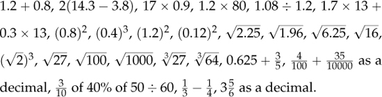
As the examples 1.4A–1.4K in Part II indicate, such mental work has clearly been undervalued in English secondary schools for some decades, with significant consequences for pupils’ subsequent progression. Here we can only illustrate what is needed on the simplest level, where pupils should be routinely expected to evaluate mentally such expressions as:
In addition to mastering simple calculation, mental and oral work is perhaps even more important, and even less common, in thinking about calculation, and numerical relations. This is indicated by the following three released items14 for Year 5 pupils from TIMSS 2001.
1.2.1A  stands for the number of pencils Pete had. Kim gave Pete 3 more pencils. How many pencils does Pete now have?
A 3 ÷ B + 3C − 3D 3 ×
1.2.1B 4 × = 28. What number goes in the box to make this sentence true?
1.2.1C 3 + 8 = + 6. What number goes in the box to make this number sentence true?
In all three cases English success rates are around, or below the international average.
1.2.1A Russia 91%,Flem Bel 85%,USA 83%,Hungary 82%,Australia 79%,England 75%
1.2.1B Russia 95%,Flem Bel 94%,Hungary 91%,USA 87%,England 82%,Australia 77%
1.2.1C Russia 80%,Hungary 50%,Flem Bel 49%,USA 47%,Australia 33%,England 29%
1.2.2The standard written algorithms need further attention at Key Stage 3 to secure their reliability for integers. More confident pupils can avoid mere repetition by concentrating on inverse problems to test their understanding (the meaning of “inverse problems” was explained in Part II, Section 1.2.3). We offer two more released items from TIMSS 2011 for Year 5 pupils as evidence that there will still be plenty to do in Year 7.
1.2.2A 5631 + 286 = …
1.2.2B 23 × 19 = …
Some will find the English success rates acceptable. But these are exercises one should expect almost all pupils to get right—as the results from other countries tend to confirm. In all cases the English performance is either below or just above the “international average”.
1.2.2A Russia 89%,USA 84%,Hungary 77%,England 67%,Flem Bel 66%,Australia 57%
1.2.2B Russia 74%,USA 59%,Hungary 40%,England 37%,Flem Bel 26%,Australia 11%
Schools who actively seek to strengthen arithmetic in Year 7 and who need harder “inverse” problems for pupils whose arithmetic is strong, could do worse than to include lots of “missing digit” problems (for example, see Tony Gardiner, Extension Mathematics Book Alpha p. 46, p. 61, p. 74, p. 125).
These written procedures then need to be extended to decimals. And the simplest calculations with decimals (such as 71.6 × 2.8, or 271.6 ÷ 2.8) demonstrate that this extension to decimals needs the corresponding integer procedures to routinely handle multi-digit inputs (at the very least 716 × 28, and 2716 ÷ 28). In the released TIMSS 2011 items at Year 9, decimal arithmetic mostly arises in context. But the following item tends to reinforce the suggestion that we currently expect too little.
1.2.2C 42.65 + 5.748 = …
1.2.2C Russia 90%,USA 89%,Hungary 88%,Australia 82%,England 79%
1.2.3At this level, calculation with fractions becomes increasingly pervasive (solving simple numerical problems involving multiplication; understanding how the standard written algorithms of column arithmetic for integers extend to those for decimals; rearranging equations and simplifying expressions; using percentages; working with ratio and proportion). And something clearly needs to change if many more pupils are to learn to calculate reliably and confidently with fractions: examples 1.4A–1.4K in Part II above suggest that we currently fail to lay the most basic foundations. Rather than offer a trite summary here, we postpone discussion of fractions until Section 1.6 below— where, as a tentative contribution to the re-thinking that is needed, we outline some of the relevant background.
1.2.4All three of the official requirements listed at the start of 1.2 include the word “use”; but the intended scope of the word is left unexplained. The official intention here may be restricted to technical usage, rather than to “applications”. But we take the opportunity to explore what it means for pupils to be able to use what they have learned.
The last 35 years have witnessed a stream of complaints that those leaving school cannot “use” what they have been certified as “knowing”. This suggests that everyone may have misunderstood what is required if a learned technique is to become available for use.
The ability to use the mathematics one knows
•includes its use within other parts of mathematics; and
•extends to simple applications, or word problems (see Section 2.3.3 in Part II for an explanation of what is meant by word problems).
In both domains, pupils’ inability to “use what they know” often has the same cause, and stems from
•the fact that a typical technique is first learned as a deterministic direct procedure,
•whereas applications frequently require a flexibility in using the procedure in the spirit of the corresponding inverse process (the distinction between direct and inverse is explained in Part II, Section 1.2.3).
In other words, pupils’ difficulties often reflect our failure to recognise the gulf between
•fluency in the underlying easy direct skill, and
•what is needed to work flexibly with this direct skill, and to handle the related inverse problems, or variations, which is what is generally needed for most applications.
Mathematics teaching and assessment have focused too strongly on the easy direct skills, and have often overlooked the fact that fluency, flexibility, and “use” require that far more attention be given to simple inverse problems. A pupil may know how to
•“find 75% of £120”
yet fail to relate this direct operation to inverse variations, such as
•“A price of £90 is raised to £120. What percentage increase is this?”, or
•“Calculate the original price if I got 25% off and paid £90”.
For each direct process, we need to allow far more time to develop the flexibility that is needed if pupils are to use the process effectively to solve related indirect problems.
1.2.5The distinction in the previous subsection is illustrated in its simplest form by the third requirement listed at the start of 1.2. Once one moves into Key Stage 3, the key to arithmetic (and later to algebra) lies in simplification. One no longer applies brute force to calculate with each expression as it is given. Instead one looks first for ways of simplifying. And the key to simplification lies in looking for
“complexifications that cancel each other out”,
that is, for hidden instances of operations cancelled out by their inverses. For example, when faced with the question:
“How many weeks are there in 50402 seconds?”
one would like pupils to set up the relevant equations
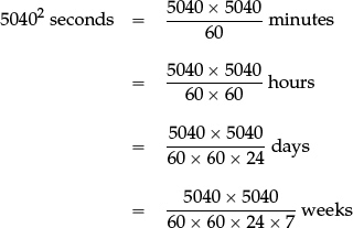
without evaluating 50402 = …, and without carrying out long divisions (or using a calculator), and then to look for ways of cancelling.
When dealing with algebraic expressions:
•It is permissible (but usually silly) to split up a single term and to spread the parts around to change a given expression into one that looks much more complicated; it is more helpful to reverse such “complexifications” by “collecting up” similar-looking terms to produce a more compact expression, which is then much easier to comprehend at a glance.
•It is equally permissible (and usually equally silly) to multiply the numerator and denominator of a given (numerical or algebraic) fraction by the same non-zero expression, and then to multiply out to make a new rational expression that appears more complicated than the original; but it is generally more sensible to factorise, to identify (non-zero) common factors, and to cancel in order to simplify.
That is,
•operations come in linked “direct-inverse” pairs which cancel each other out (addition-subtraction; multiplication-division; powers-roots; multiplying out and factorising; etc.).
Simplification is essentially the art of spotting such combinations, and cancelling them out.
This key algebraic art needs to be exercised and mastered first within arithmetic—so that numerical expressions are no longer “blindly evaluated”, but are routinely simplified, using what we have called structural arithmetic (see Part II, Section 2.1.1)—so that one routinely notices: that
28 + 186 + 72 = (28 + 72) + 186 = 286;
or that
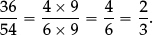
One is then in a position to be pleasantly surprised by equivalences that are less obvious (such as that  ).
).
1.2.6The first of the requirements listed at the start of 1.2 refers to “proper and improper fractions” and to “mixed fractions”. The expressions “proper fraction” and “improper fraction” make sense in Key Stage 2, but they are no longer really appropriate at Key Stage 3.
Fractions are introduced in Key Stage 1 and Key Stage 2 as parts of a whole, and so are automatically less than 1; hence, at that stage, when one comes to refer to fractions that are greater than 1, it makes sense to call them “improper”. But the distinction is not a mathematical distinction; it arises because of the way fractions are introduced.
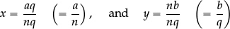
From Key Stage 3 onwards all fractions, whether greater than 1 or less than 1, should be treated in the same way, as the quotient of two integers  , with q > 0. Hence the use of words like “proper” and “improper” should be left behind (along with such language as “timesing”).
Similarly, though it may sometimes be appropriate to present an answer in “mixed” form (say as  ), the expression “mixed number” is out of place in secondary mathematics.
1.3.[Subject content: Number p. 6]
–use a calculator and other technologies to calculate results accurately and then interpret them appropriately
“Calculators and other technologies” were first advocated at secondary level some 40 or more years ago. Yet we still do not seem to have forged a consensus as to when their use is “appropriate”, and when not.
The opening Aims (see page 2 of the National Curriculum programmes of study for Key Stage 3) include the sensible warning that calculators, etc.
“should not be used as a substitute for good written and mental arithmetic” [emphasis added].
However, this sound advice still needs to be interpreted. And the positive guidance as to when calculator use is “appropriate” is only slightly more helpful. The general advice offered at the beginning of the programmes of study for Key Stages 1 and 2, on pages 3 and 4,15 says that calculators should only be introduced
“to support pupils’ conceptual understanding and exploration of more complex number problems, if written and mental arithmetic are secure” [emphasis added].
The dilemma highlighted by this advice refers to integer arithmetic in primary schools. But the same dilemma recurs throughout Key Stage 3—with decimal arithmetic, with fractions, with surds, and so on. Secure calculation by hand and in the head is a crucial ingredient of the way beginners internalise meaning, structures, and procedures. So in each case the above instruction would seem to imply that
•pupils should achieve conceptual understanding and mental and written fluency before routinely using a calculator,
•but that once a suitable level of fluency has been achieved, one can safely delegate “more complex number problems” to the calculator, and exploit the power of the calculator to extend conceptual understanding into new realms (see the example at the end of this section).
The introduction to the programmes of study for Key Stage 1 and 2 and for Key Stage 3 both state that
“In both primary and secondary schools, teachers should use their judgement about when ICT tools should be used.”
But the wider community remains confused. The judgement in the previous paragraph (that “secure calculation is an important part of the way beginners internalise meaning”) would seem to be a reasonable summary of views in many other countries. But teachers in England will know that the mathematics education community here remains divided. Hence teachers must be prepared to develop and to use their own judgement as they are exhorted to do.
To illustrate the divide, we give just two recent examples. The first is a report published by the Joint Mathematical Council16 and a riposte.17 The second is a debate between a strong advocate of “computer based mathematics” in schools and an agnostic:18 (see “Technology and maths”).
Technology is clearly seen as “sexy” by politicians and by enthusiasts. And its evident potential should certainly be explored. But it is not easy for ordinary teachers to see beyond the rhetoric in order to discern
•whether we have already discovered some magic “royal road” to elementary mathematics, that removes the need for beginners to master the art of hand calculation; or
•whether those who currently advocate increased use of technology by beginners are getting ahead of themselves, and are misleading the rest of us as to what is currently in pupils’ interests.
Whatever may be the eventual impact of technology on the learning of mathematics, the present evidence from international studies (illustrated by examples 1.4A–1.4K in Part II) would seem to be that we in England have tended to delegate calculation to the calculator or computer far too easily. Instead of using technology to achieve more, we have used it as a convenient alternative to achieving meaning and mastery. That is, we have failed to heed the exhortation of the official programme of study, and have allowed technology to be “used as a substitute for” pupils’ understanding of written and mental arithmetic.
Computation by hand, or in the head, has too often been repudiated as if it were merely outmoded drudgery, or some puritanical hangover. But the importance of calculation at all levels stems from the role played by mental and written procedures in the subtle process of human sense-making. So we should perhaps hesitate before discarding it until such time as we are sure that we have other ways of establishing the kind of meaning that will allow pupils to use elementary mathematics with confidence.
The requirement that pupils should “use calculators and other technologies”
“to calculate results accurately and then interpret them appropriately” [emphasis added]
needs to be interpreted with care. A calculator certainly allows us all to work with messier numerical data than we could otherwise manage. But for most calculations, a calculator is the opposite of “accurate”: its value lies in the fact that it is “quick and dirty”, and produces an answer which is a very good approximation, but which may not be exact. The ubiquity of calculators, and their ease of use makes it important for pupils to develop their own internal sense of number so that they can use calculators intelligently, interpret the approximate answers which they produce, and use these tools to extend their own powers of analysis.
To give an example from within elementary mathematics (having one eye on the next subsection), one might invite more able pupils in Year 8 or Year 9 to work (initially without a calculator) to address these three questions:
Find a prime number which is one less than a square. | |
Find another such prime number. And another. | |
How many such prime numbers are there? |
Different teachers will exploit the proposed task in different ways. Pupils must first access whatever internal register of squares they have, and then reinforce and extend their internal list to generate:
(12 − 1 = 0,) 22 − 1 = 3, 32 − 1 = 8, 42 − 1 = 15, 52 − 1 = 24, 62 − 1 = 35, 72 − 1 = 48, 82 − 1 = 63, 92 − 1 = 80, 102 − 1 = 99, 112 − 1 = 120, 122 − 1 = 143, 132 − 1 = … , …
They must then decide which of these numbers are prime. The associated “noise” (of having first to think about squares, then to subtract 1) makes this more awkward than simply asking pupils to test given integers to see whether they are prime. So one can anticipate some surprising mistakes. For example: though 8, 15, 24, 35, 48 are unlikely to be labelled as primes, the surrounding “noise” means that part (b) may well lead to 63 and 143 being proposed as candidate primes.
There are challenges here for pupils on many levels. A calculator may at first be used simply to extend the list of squares. If so, then 168, 195, 224, 255, 288, 360, 440 are unlikely to be proposed as primes; but 399 and 483 might well be, and 323 will almost certainly feature.
However, once the proposed candidates 63 (= 7 × 9), 143 (=11 × 13), and 323 (= … × …) have been seen to fail, one would like pupils to think rather than just press buttons and guess. A mixture of patience and prodding should allow them to discover the apparent pattern
8 = 2 × 4,
15 = 3 × 5,
24 = 4 × 6, etc.,
and they can then to use the distributive law to multiply out
(n − 1)(n + 1) = n(n + 1) −1(n + 1) = n2 + n − n − 1 = n2 − 1,
and to discover
•the advantages of thinking and working with symbols (“n2 − 1”)
•rather than with words (“one less than a square”).
1.4.[Subject content: Number p. 5]
–use the concepts and vocabulary of prime numbers, factors (or divisors), multiples, common factors, common multiples, highest common factor, lowest common multiple, prime factorisation, including using product notation and the unique factorisation property
–use integer powers and associated real roots (square, cube and higher), recognise powers of 2, 3, 4, 5 and distinguish between exact representations of roots and their decimal approximations
This collection of topics related to integer arithmetic deserves to be taken more seriously than has perhaps traditionally been the case at secondary level. The following released item from TIMSS 2011 for pupils in Year 9 suggests that work on primes and factors from primary school is often not followed up.
1.4A Which of these shows how 36 can be expressed as a product of prime factors?
A 6 × 6B 4 × 9C 4 × 3 × 3D 2 × 2 × 3 × 3
1.4A Hungary 69%,Russia 68%,USA 64%,England 51%,Australia 45%
Bare hands integer arithmetic may suffice for pupils to find HCFs (to cancel fractions), and LCMs (to add or subtract fractions by writing both with a common denominator). But if the official requirements are interpreted coherently, then the listed ideas constitute a valuable “Key Stage 3 introduction to Number theory”, a subject which is increasingly important in a world dominated by “calculators and other technologies”.
1.4.1The second listed requirement in 1.4 “use integer powers” is perhaps the simplest starting point. Pupils should recognise and work with
squares: 12 = 1, 22 = 4, 32 = 9, 42 = 16, 52 = 25, 62 = 36, 72 = 49, 82 = 64, 92 = 81, 102 = 100, 112 = 121, 122 = 144, … ;
and
cubes: 13 = 1, 23 = 8, 33 = 27, 43 = 64, 53 = 125, 63 = 216, … , 103 = 1000.
They should also recognise the powers of 10 in exponent form and know the corresponding values:
powers of 10: 10, 102 = 100, 103 = 1000, 104 = 10000, 105 = 100000, 106 = 1000000, etc.
And they should work with and recognise powers of small integers, such as:
powers of 2: 2, 22 = 4, 23 = 8, 24 = 16, 25 = 32, 26 = 64, 27 = 128, 28 = 256, 29 = 512, 210 = 1024
powers of 3: 3, 32 = 9, 33 = 27, 34 = 81, 35 = 243
powers of 4: 4, 42 = 16, 43 = 64, 44 = 256, 45 = 1024
powers of 5: 5, 52 = 25, 53 = 125, 54 = 625.
Squaring is a “unary operation” or function (in that the output n2 is uniquely determined by a single input). Once sufficiently many squares are known, they can be exploited to interpret the exact meaning of the inverse unary operation, that is the square root function  where
where
 denotes “the positive number whose square is equal to n”.
Notice that, since is to be a function,  must denote a unique value—namely the positive number whose square is equal to 4: i.e. 2. In contrast, the quadratic equation “x2 = 4” has two solutions, which are ±.
Later, appropriate groups of pupils can help to formulate and prove:
Claim If a2 = b2, then a = ± b.
Proof Suppose a2 = b2.
∴ a2 − b2 = 0
∴ (a − b)(a + b) = 0
∴ a − b = 0, or a + b = 0, so a = ± b. QED
This shows that there is just one positive number whose square has a given positive value.
Provided n is a perfect square, pupils can find the exact value of : for small squares:

and for larger squares:

They may be encouraged to notice that

and that
They can then use this as a short cut to find the square root of larger squares such as  .
.
[Later they can prove that:
Claim  whenever a and b are positive:
Proof  is clearly positive (since
  and
and  are both positive).
And 
And once sufficiently many cubes are known, pupils can find  when n is a perfect cube:

With help they may notice that

This basic repertoire of calculations using powers and roots can then develop in two very different directions—one focusing on calculation, and the other on structure.
1.4.2Further calculation The notation  and
and  for square roots and cube roots has many features in common with the notation for fractions.
Some fractions, like  = 4, or
  = 0.25, stand for familiar numbers, and can be exactly evaluated. But most fractions one can write down (such as
  ≈ 0.167) do not stand for any otherwise familiar number, and cannot be evaluated exactly. The value of the fraction notation is that it provides a way of writing exact expressions for “ideas of numbers”, which we often have no other way of writing exactly, such as
“that number—six identical copies of which add up to 1”.
Similarly, the functions and  allow us to write exact expressions for numbers, most of which cannot be evaluated exactly as decimals, or in any other way. We know that
  = 2. But what number is represented by
  ? Or by
  ? Or by
  ? Or by
  ? Or by
  ?
?
Before we worry about the square root of fractions or decimals, there is plenty of work to be done to establish the meaning and the arithmetical rules for working with surds: that is numbers of the form  when n is an integer. For example, we need to ensure
•that  is understood formally to be “the (positive) number whose square is 10”;
•that since 10 lies between 9 and 16,  is seen to be slightly bigger than
  = 3 (and a lot less than
  = 4);
= 4);
•that pupils compare the side length of a square of area 10 square units, with that for a square of area 9, and one of area 16; and
•that they later compare the length of a diagonal of a 1 by 3 rectangle
with the length (= 3) of the longest side, and | |
with the length (= 4) of the route round the perimeter of the rectangle from one corner to the opposite corner. |
These ideas can later be taken further. Pythagoras’ Theorem shows that an isosceles right angled triangle with legs of length 1 has a hypotenuse of length exactly  . The hypotenuse is clearly longer than each of the two legs; and the triangle inequality shows that the hypotenuse is less than the sum of the two shorter sides. So we know that 1 < < 2. But to pin down the value of more accurately requires us to use a little of what we know about integer squares:
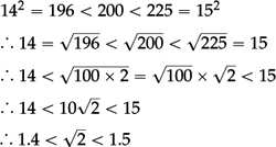
[In short: 1.42 = 1.96 < 2, and 1.52 = 2.25 > 2.]
Similarly, Pythagoras’ Theorem shows that an equilateral triangle of side 2 has height exactly  , and that this height is less than the hypotenuse, so < 2; and the triangle inequality shows that 1 + > 2. Hence 1 < < 2. But to pin down the value more accurately we have to use what we know about integer powers to find reasonable estimates:
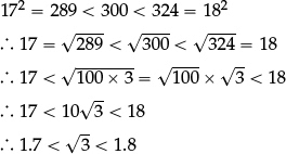
[In short: 1.72 = 2.89 < 3, and 1.82 = 3.24 > 3.]
In the same way one can use what pupils know about perfect cubes to ensure
•that  is interpreted as “the number whose cube is equal to 10”;
•that this number is seen to be slightly bigger than  = 2 and considerably smaller than
  = 3;
= 3;
•that pupils compare an imagined cube of volume 10 cubic units with a smaller cube of volume 8 and a larger cube of volume 27 cubic units—noting and understanding how a modest increase in the edge length leads to a cube with three times the volume!
1.4.3Structure: the index laws The structural (or algebraic) theme related to powers prepares the ground for the index laws. The index laws are not explicitly mentioned within the Key Stage 3 programme of study, but there are several reasons why they need to be squarely addressed at this level.
One reason is that, as we shall see in Section 1.5, zeroth and negative powers are needed to represent real numbers in standard form; and the way we define these powers only really makes sense if we think in terms of the advantages of “preserving the index laws”.
A more basic reason is for pupils to understand why
when we multiply a digit in the 10m place (or column) by a digit in the 10n place (or column), the answer belongs in the 10m + n column.
For this to make sense, pupils already need to know in their bones how products of powers work: for example, that
102 × 105 = (10 × 10) × (10 × 10 × 10 × 10 × 10) = 102+5, and 22 × 25 = (2 × 2) × (2 × 2 × 2 × 2 × 2) = 22+5.
Once pupils
•think of the place value of positions, or columns, in terms of the exponent of the “power of 10”, rather than verbally as “units, tens, hundreds, etc.”, and
•realise that “when we multiply powers, we add exponents”,
it becomes natural to think of the unit as 100 = 1.
The rightmost place when representing an integer then corresponds to the “(units digit) ×100”.
The fact that 100 = 1 then fits in with the way powers multiply (since we want 101 × 100 = 10(1+0) = 10).
Once the units column (just to the left of the decimal point) is associated with 100, it becomes plausible that the place immediately to the right of the decimal point might correspond to “10−1”. And the idea that “when we multiply powers, we add exponents” also helps to explain why we take “10−1” to equal  (since we want: 101 × 10−1 = 101 + (-1) = 100 = 1 = 10 ×
  ).
).
1.4.4Introduction to number theory It is easy to compare, and to add, two fractions with the same denominator; but it is not at all obvious how to compare, or to add, two fractions with different denominators m, n. However, as soon as we change each fraction to one that is equivalent to it, and which has denominator “LCM(m, n)”, comparison is again immediate, and addition, subtraction and division can be carried out easily. Hence LCMs come into their own as soon as we wish to compare, or to add, subtract, or divide two fractions with different denominators m and n. In general HCFs and LCMs feature whenever a problem requires us to switch to a common unit that works for both m and n (whether a multiple of each, or a submultiple—or factor—of each).
The HCF and LCM of two given integers m, n are easy to find in a primitive way.
HCF: Each of the given integers m, n has a finite number of factors, and these can be listed; the two lists can then be scanned to find the “highest”, or largest, factor in both lists.
LCM: The LCM of the given integers m, n can be found by making a list of (positive) multiples of each number (2m, 3m, 4m, … ; and 2n, 3n, 4n, …) and looking for the “least” multiple that occurs in both lists.
These primitive approaches are easy to implement, but are slightly unwieldy. Moreover, they do not immediately suggest, or explain why it is always true that:
HCF(m, n) × LCM(m, n) = m × n.
For suitable groups of pupils it is worth making sure that this result is discovered, or at least noticed, and if possible proved.
[Proof Let HCF(m, n) = h.
∴ m = h × m′ and n = h × n′, where m′ and n′ have no common factors.
∴ m′ × n = m′ × (h × n′) = (m′ × h) × n′ = m × n′ is a multiple of m and of n, so is a common multiple of both m and n.
The fact that it is the LCM follows from the important fact that every common multiple of both m and n is also a multiple of their LCM. (So if there were a smaller common multiple of m and n, say k, then it would have to be a proper factor of m′ × h × n′ and the quotient would be a factor of both m′ and n′.)
∴ HCF(m, n) × LCM(m, n) = h × (m′ × n) = (h × m′) × n = m × n. QED]
The observation that LCM(m, n) is a factor of every common multiple of m and n is not hard, but cannot easily be proved at this level. However, it can be established as a “fact of experience” by listing the common multiples of suitable pairs, such as:
2 and 3:6, 12, 18, 24, …
6 and 8:24, 48, 72, 96, …
6 and 14:42, 84, 126, …
30 and 42:210, 420, 630, … .
And the fact that
HCF(m,n) × LCM(m,n) = mn
can be re-explained later when one is in a position to look at HCFs and LCMs in terms of the prime factorisations of the two integers m and n.
The Key Stage 3 requirements relating to prime numbers and prime factorisation extend what is expected at Key Stage 2. There we find that pupils (in Year 5) are supposed to
•“know and use the vocabulary of prime numbers, prime factors and composite numbers”
•“establish whether a number up to 100 is prime and recall prime numbers up to 19”, and
•“recognise and use square numbers and cube numbers and the notation for squared (2) and cubed (3)”.
Although we have been told that “Key Stage 3 should build on Key Stage 2”, it may be wise to revisit, and to reinforce, these ideas in Year 7 before ploughing ahead (especially with regard to the third bullet point, which seems unnecessarily premature). A sensible initial goal at Key Stage 3 is
•to get to know the twenty five prime numbers up to 100
by implementing the Sieve of Eratosthenes (Greek, 3rd century BC).
•Write out the integers 1–100 in ten columns. Cross out 1 (as 1 is not a prime).
•Circle the first uncrossed integer (the prime 2) and cross out all its larger multiples.
•Circle the first uncrossed integer (the prime 3) and cross out all its larger multiples.
•Circle the first uncrossed integer (the prime 5) and cross out all its larger multiples.
•Circle the first uncrossed integer (the prime 7) and cross out all its larger multiples.
Then check that all of the remaining uncrossed integers
11, 13, 17, 19, 23, 29, 31, 37, 41, 43, 47, 53, 59, 61, 67, 71, 73, 79, 83, 89, 97
are in fact primes. (The reason why should be revisited later when the “square root test” has been understood—see later in this section.)
As part of this exercise one would like pupils to learn that, although unfamiliar integers sometimes “smell like a prime”, this may be simply because (like 51, or 91, or 323) they are not routinely encountered in the multiplication tables. Pupils will later need to develop a systematic way of testing any three-digit integer to see whether it is prime (the “square root test”).
The programme of study includes “prime factorisation” as an explicitly declared goal. So it is important to explain why we do not count “1” as a prime number (and to make it clear that this has nothing to do with enforcing an arbitrary definition of a “prime” as an integer with “exactly two factors”). Pupils should understand (from their own extensive experience of factorising integers: see below) that
•prime numbers are the “multiplicative atoms” for integers.
Hence we can break up any given integer as the product of its constituent prime factors. Once we grasp this important property of prime numbers, it should be clear that “1 is different”, e.g.
1 = 1 × 1 = 1 × 1 × 1 = …,
2 = 2 × 1 = 2 × 1 × 1 = 2 × 1 × 1 × 1 = ….
So “1” is not such a constituent atom, and it would simply get in the way if we made the mistake of calling it a prime.
Some thought is needed when choosing a systematic procedure for “factorising integers”. “Factor trees” may have a place for beginners, but it is worth thinking carefully why they are best left behind when we come to Key Stage 3 (along with oblongs, timesing, improper fractions, and mixed numbers). The most suitable systematic algorithm for achieving prime factorisation of a given integer is to carry out successive short divisions—upside down:
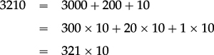
“Write 2310 as a product of prime powers.”
2 is clearly a factor of 2310: 
∴ 2310 = 2 × 1155
3 is clearly a factor of 1155: 
∴ 2310 = 2 × 1155 = 2 × 3 × 385
5 is clearly a factor of 385: 
∴ 2310 = 2 × 3 × 5 × 77
7 is clearly a factor of 77: 
∴ 2310 = 2 × 3 × 5 × 7 × 11
If we apply a slightly compressed version of the same procedure to less carefully chosen starting integers—such as 1234, or 12345, or 123456, or 4321, or 54321, or 654321, then we quickly discover the need for an efficient way of deciding whether “large” integers are prime.
 ∴ 1234 = 2 × 617. But is 617 prime?
12345: 5 is clearly a factor:
 ∴ 12345 = 3 × 5 × 823. But is 823 prime?
123456: 2 is clearly a factor:
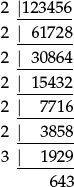 ∴ 123456 = 26 × 3 × 643. But is 643 prime?
These unanswered questions lead naturally to the square root test for deciding whether a given integer is prime:
Square root test: Suppose that 643 is not prime.
Then 643 factorises—say as 643 = a × b, where a, b are both “proper factors” (i.e. a, b > 1) We may choose a to be the smaller of the two proper factors: so 1 < a ⩽ b.
Then
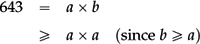
∴  , so the smaller factor a ⩽
  < 26.
< 26.
Hence to test whether 643 is prime, we only need to test for factors up to 25.
The first few short divisions can be done in the head:
2 is clearly not a factor of 643;
3 is not a factor (the simple ‘divisibility tests’ are discussed below);
(4 cannot be a factor—or else 2 would have been a factor);
5 is clearly not a factor;
(6 cannot be a factor or else 2 and 3 would have been factors);
7 is not a factor;
(8 cannot be a factor or 2 would have been a factor; similarly 9 and 10 cannot be factors);
11 is not a factor; and so on.
The reasons why we do not have to check 4, 6, 8, 9, 10, … show that we only have to check for possible prime factors up to  —that is up to 23. And once the easy short divisions have been checked, it makes perfect sense to use a calculator to test for larger possible prime factors (say beyond 7, or 11). Moreover calculator use makes the power and speed of the method even more evident:
643 ÷ 13 = 49.46…;
643 ÷ 17 = 37.82…;
643 ÷ 19 = 33.84…;
643 ÷ 23 = 27.95….
∴ 643 is prime
Pupils can now look back at the “sieve of Eratosthenes” for the integers 1–100 and understand why it stopped at multiples of 7:
Proof Any non-prime ⩽ 100 must have a prime factor ⩽  = 10.
= 10.
That is, every non-prime ⩽ 100 is a multiple of 2, or of 3, or of 5, or of 7. QED
Armed with this method, they can then complete a “sieve of Eratosthenes” to find all prime numbers up to 500 (by following the same procedure—circling the first uncrossed number and crossing out all higher multiples—for primes up to  = 22.36…—that is up to 19). Hence, in order to extend the list from 100 to 500 we only need to carry out four extra steps, to eliminate multiples of 11, of 13, of 17, and of 19.
The fact that every positive integer can be factorised in just one way as a product of prime powers cannot be proved at this level. Instead the uniqueness of prime factorisation emerges as a “fact of experience”: the factorisation procedure above churns out the prime factorisation each time, and the subtle question as to its uniqueness is unlikely to arise.
There is plenty of mileage in exploiting prime factorisation. For example:
•to recognise squares as precisely those integers whose prime factorisation only involves primes to even powers
•to recognise cubes as precisely those integers whose prime factorisation only involves primes raised to powers that are all multiples of 3
•to see how HCF(m, n) is just the product of those prime powers that occur both in the prime factorisation of m and in the prime factorisation of n, and hence to re-prove
HCF(m, n) × LCM(m, n) = m × n.
Divisibility tests are not explicitly mentioned in the Key Stage 3 programme of study. However, the requirements to understand place value (Section 1.1) and to test for factors (Section 1.4) should highlight the need to discuss these excellent examples of structural arithmetic.
The fact that multiples of 10 are precisely the integers having “units digit = 0” is an evident consequence of place value: for example
Any integer N can therefore be decomposed as “a multiple of 10” plus its “units digit”. The first of these two terms “a multiple of 10” is also “a multiple of 2” (because 10k = (2 × 5)k = 2 × (5k)).
∴ An integer N is a multiple of 2 precisely when its units digit is a multiple of 2.
That is, when it ends in 0, 2, 4, 6, or 8. (Be prepared to have to insist that “0 = 0 × 2” is a multiple of 2, and so is even.)
Similarly, any multiple of 10 is also a “multiple of 5” (because 10k = (5 × 2)k = 5 × (2k)).
∴ an integer is a multiple of 5 precisely when its units digit is a multiple of 5.
That is, when it ends in 0, or 5.
The same idea shows that multiples of 100 are precisely the integers having “both tens and units digits = 0”.
Any integer N can be decomposed as “a multiple of 100” plus the number formed by its tens and units digits. The multiple of 100 is also a “multiple of 4” (because 100k = (4 × 25)k = 4 × (25k)).
∴ N is a multiple of 4 precisely when “the number formed by its last two digits is a multiple of 4”.
Multiples of 1000 are precisely the integers having hundreds, tens and units digits = 0.
Any multiple of 1000 is also a “multiple of 8” (because 1000k = (8 × 125)k = 8 × (125k)); so an integer is a multiple of 8 precisely when “the number formed by its last three digits is a multiple of 8”.
This shows how the rules for spotting multiples of 2, or 4, or 5, or 8, or 10 derive from our place value system for writing numbers.
The divisibility tests for multiples of 3, and of 9 depend on the place value system in a more interesting way, which obliges us to think about the algebraic structure of the place value system. The key here lies in the fact that
10 − 1 = …, 100 − 1 = …, 1000 − 1 = … etc. are all multiples of 9.
Later this can be seen as a special case of the beautiful factorisation
xn − 1 = (x − 1)(xn − 1 + xn − 2 + xn − 3 + … + x + 1).
Hence any integer such as 12345, can be deconstructed into
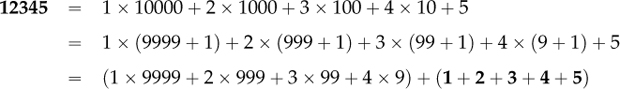
The first bracket is clearly a multiple of 9—and so is also a multiple of 3.
Hence, for 12345 to be a multiple of 3 the second bracket—that is, its digit-sum “1+2+3+4+5”—must be a multiple of 3 (which it is!).
And for 12345 to be a multiple of 9, the second bracket—that is, its digit-sum “1+2+3+4+5”—must be a multiple of 9 (which it is not). This yields a simple (and intriguing) test for divisibility by 3 and by 9.
The test for divisibility by 6 is mildly different: an integer is divisible by 6 precisely when it is divisible both by 2 and by 3. Similarly, an integer is divisible by 12 precisely when it is divisible both by 4 and by 3. Here it is important that HCF(3, 4) = 1. (Notice that 18 is a multiple of 6 and of 9; but 18 is not a multiple of 6 × 9 = 54, because HCF(6, 9) ≠ 1.)
Divisibility by 11 = 10 + 1 depends on a simple variation of the reasoning for divisibility by 9 = 10 − 1. The key here lies in the fact that
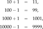
etc. are all multiples of 11.
An interesting consequence of the prime factorisation of an integer is that it allows an easy way of counting the number of factors which the integer has without listing them all first. The idea depends on “the product rule for counting” which is needed at Key Stage 3—but is not explicitly mentioned. However, it is optimistically hinted at rather vaguely in the Year 6 programme of study under
“Algebra: – enumerate possibilities of combinations of two variables”.
And the product rule is explicitly required at Key Stage 4.
The simplest version of the product rule tells us that the number of dots in a rectangular array is equal to “the number of dots in each row times the number of rows”.

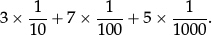
Instead of counting the dots individually, we note that there are 3 rows, each with 7 dots, so the total number of dots is “7 + 7 + 7 = 3 × 7”.
A similar situation arises whenever we are effectively counting “ordered pairs”. When we roll two dice, one red and one blue, each outcome can be listed systematically as an ordered pair:
(red score, blue score).
The key observation is that each possible first coordinate has the same fixed number of possible second coordinates, so the total number of outcomes can be counted very easily.
There are 6 possible red scores;
and each red score can occur with each of the 6 possible blue scores;
so there are
6 + 6 + 6 + 6 + 6 + 6 = 6 × 6
possible ordered pairs, or outcomes for rolling the two dice.
In the same way, if we want to count the possible factors of 12 = 22 × 3, then each factor must have the form 2a × 3b with a = 0, 1, or 2, and b = 0, or 1. So
there are 3 possible choices for a;
and for each choice of a there are 2 choices for b. ∴ 3 × 2 possible factors:
20× 30 = 1, 20× 31 = 3, 21× 30 = 2, 21× 31 = 6, 22× 30 = 4, 22 × 31 = 12.
1.5.[Subject content: Number p. 5]
–understand and use place value for decimals, measures and integers of any size
–interpret and compare numbers in standard form A × 10n, 1 ⩽ A < 10, where n is a positive or negative integer of zero
The two requirements in 1.5 are closely intertwined—even if the second bullet point seems slightly premature from a purely mathematical viewpoint. (Standard form may have been included at this level to support the requirements of science teaching. Yet there is no mention of “standard form” in the Key Stage 3 science programme of study—unless the numerical significance of the “pH scale” as
“the decimal logarithm of the reciprocal of the hydrogen ion activity in a solution”
is to be explained in detail, or the value of “Newton’s gravitational constant” is to be pulled out of a hat as “≈ 6.67 × 10⁻¹¹N · (m/kg)2”.)
The sequence of topics related to the requirements in 1.5 would seem to include:
•understanding and working with positive integer powers
•recognising that multiplication of powers of 10 corresponds to “adding exponents” (i.e. the index laws)
•understanding that defining “100 = 1” is consistent with the place value notation for integers (so that the tens column is in some sense the 1st column, and the units column is the “zeroth” column), and that this definition of 100 preserves the index laws for multiplication (103 × 100 = 10(3+0) = 103)
•understanding that defining “10−n” to be equal to the reciprocal of 10n then allows us to interpret the decimal places to the right of the decimal point in the same way (as the “(−1)th” column, the “(−2)th column”, the “(−3)th column”, the “(−4)th column”, and so on), and that this also respects the index laws
•learning to write any integer with n + 1 digits as a decimal A (1 ⩽ A < 10) multiplied by 10n (by moving the decimal point n places to the left to follow the leading digit), and learning to translate numbers which are given in standard form back into their more familiar guise
•extending this notation to numbers which are less than 1, so that it can be used for all positive real numbers
•learning to compare numbers given in standard form
•learning to interpret the conventions associated with rounding, where numbers are specified to so many “significant figures”, or to so many “decimal places”
•learning how to multiply and divide, and to add and subtract, numbers given in standard form (bearing in mind the specified levels of accuracy).
Experience with different groups of pupils will determine which parts of this sequence are better delayed until Year 10 (or even Year 11). For example, some pupils may be able to compare relatively simple examples of numbers given in standard form, but will need to revisit and extend the idea in Years 10 and 11. However, the final bullet point in the sequence seems much too demanding at this stage, since it involves the interaction between standard form and rounding, or approximation. (Numbers given in standard form are almost never exact. So arithmetic with numbers given in standard form needs to be linked with an understanding of numerical data being “accurate to so many decimal places”, and with the use of “significant figures”.)
The first few bullet points in the above sequence were incorporated in our comments on powers in Section 1.4. On one level, in order to understand that
it is enough to know that
3.1 × 10 = (3 + 0.1) × 10, and that
0.1 is equal to  (that is, that the “1” in the first decimal place corresponds to “tenths”).
However, the general procedure for interpreting standard form makes much more sense once it is clear that the digit that is k places to the right of the decimal point corresponds to a multiple of 10−k, so that multiplying by a suitable power of 10 simply “moves the decimal point” that number of steps to the right (or keeps the decimal point fixed and moves the digits the same number of steps to the left).
The same ideas are worth addressing because they are needed to understand
•the way division by a decimal can be transformed into division by an integer (by multiplying both the divisor and the dividend by a suitable power of 10), and
•the way multiplication of decimals can be transformed into a three-step process
–first multiplying by a suitable power of 10 to transform the calculation into a familiar multiplication of integers,
–then carrying out the multiplication of integers,
–then dividing by the same power of 10 (that is, re-positioning the decimal point in the answer) to find the required answer.
Hence it may well be possible to convey something of the meaning of the standard form notation before the end of Key Stage 3—at least for those who are likely to need it elsewhere. But, in the spirit of the declared Aims of the mathematics programme of study, we urge mathematics teachers to avoid simply presenting standard form as an uncomprehended formalism. Instead we hope schools will lay the necessary foundations in Year 7 and 8 (through exercises that expand and then simplify powers such as
102 × 105 = (10 × 10) × (10 × 10 × 10 × 10 × 10) = 102+5,
linking this to an understanding of long multiplication), so that some modest version of the notation can be properly understood in Year 9 say. (The index laws offer a rare opportunity for pupils to experience at first hand the way meanings and definitions are extended in mathematics, though this opportunity is generally missed. For a systematic development at this level see Extension mathematics Book Gamma (Oxford 2007), Sections T14, C24, C31, C38.)
However, before launching into standard form, it would be good if pupils understood why it is often helpful to think in terms of “powers of 10”, and why we focus on the exponent (or “baby logs”) when dealing with very large or very small quantities or measurements. An easily available point of entry would be to watch the classic short movie Powers of 10, made many years ago by the Eames brothers.19 (The film invites repeat viewing, stopping from time to time to discuss what is being shown.)
One everyday instance, where we focus on the exponent (or the logarithm) rather than the number itself, arises with the Richter scale for measuring the strength of earthquakes. This may already be familiar to some pupils. Here an increase of 1 in the measurement used on the Richter scale corresponds to an earthquake which is 10 times more powerful, and an increase of 2 corresponds to an earthquake which is 100 times more powerful. Other instances where such “log-scales” are used include the measure for the brightness of stars, and the pH scale.
1.6.[Subject content: Number p. 5]
–use the four operations […] applied to […] fractions
–work interchangeably with terminating decimals and their corresponding fractions (such as 3.5 and  , or 0.375 and
  )
)
–define percentage as ‘number of parts per hundred’, interpret percentages and percentage changes as a fraction or a decimal, interpret these multiplicatively, express one quantity as a percentage of another, compare two quantities using percentages, and work with percentages greater than 100%
–interpret fractions and percentages as operators
–[Ratio, proportion and rates of change p. 7] solve problems involving percentage change: including percentage increase, decrease and original value problems; and simple interest in financial mathematics
As the last listed item here indicates, the boundary between this section and Section 1.9 below (on ratio and proportion) is blurred—so the two need to be considered together. The first listed requirement concerning calculation with fractions was also considered briefly in Section 1.2. However, since achieving fluency in calculating with fractions should be a central goal of Key Stage 3, this deserves to be addressed here in greater detail than was possible as part of Section 1.2.
1.6.1Fractions as a unifying idea The central importance of calculation with fractions for all pupils only becomes apparent in late Key Stage 3 and early Key Stage 4. Before that pupils learn to work with division (sharing and grouping), parts of a whole, decimals, fractions, ratios, percentages, proportion, scale factors—first numerically and then within algebra. But at some stage pupils ideally discover that all of these apparently different ideas and procedures reduce to “calculation with fractions”.
1.6.2Prerequisites and follow-up When preparing to address the arithmetic of fractions in early Key Stage 3, the first move should be a check that the necessary prerequisites from integer arithmetic are firmly in place. These include: complete arithmetical fluency with integers; and flexibility in identifying common multiples (in order to switch to common denominators), and in identifying common factors (in order to simplify by cancelling).
The subsequent developments summarised below constitute a considerable challenge. But such examples as 1.4C, 1.4F, and 1.4H in Part II suggest rather clearly that the arithmetic of fractions needs to be given more time than has been usual in recent years. In particular, fraction work should be routinely included as part of solving equations, solving word problems, finding equations of straight lines through given points, and within other applications during the ensuing 2–3 years (where it has often been artificially avoided by restricting to problems with small integer solutions).
1.6.3Fractions as operators and percentages The fourth requirement listed at the start of 1.6 reads as though pupils start out with a clear understanding of “fractions as numbers”, and then need to interpret these “numbers” as “operators”. This is potentially misleading.
Fractions are initially introduced (in Key Stages 1 and 2) as “parts of a whole”—that is, as [implicit] “operators”. At that stage pupils have no conception of fractions as numbers, such as  or
or  , but work only with “parts of an understood whole”.
At some point these “parts of a whole”, such as “half a pint” or “three quarters of a cake”, have to give birth to the numbers and . Exactly how this shift from working with “parts of a given whole” to “fractions as numbers” is supposed to be made is never clarified in the Key Stage 2 programme of study. So we may anticipate that many pupils entering Key Stage 3 will still think of fractions only as operators (so the word “fraction” will immediately conjure up the idea of “a fraction of” some whole).
The third, fourth and fifth requirements listed in 1.6 refer to percentages. The key here is to recognise that all work with percentages should eventually reduce to a particular instance of work with fractions (sometimes in decimal form). That is, “percentages” should eventually be no longer seen as a separate topic, and fractions (and their arithmetic) should become the unifying theme. We make three further comments on percentages.
First, once the transition from “fractions as operators” to “fractions as numbers” has been firmly established, pupils need to re-interpret fractions as “operators” once again, in order to implement the standard applications efficiently—so that, for example, a “20% increase” is naturally calculated by multiplying by 1.2, rather than by calculating 20% and adding.
The second comment on percentages has already been made in Section 1.2.3 of Part II, and in Section 1.2.4 above, but bears repetition in the context of percentages. Mathematics teaching and assessment too often focus on the easy direct skills, and overlook the fact that fluency, flexibility, and “use” generally require that far more attention needs to be given to simple inverse problems. A pupil may know how to
•“find 75% of (i.e. three quarters of) £120”
yet fail to relate this direct operation to the different inverse variations, such as
•“A price of £90 is raised to £120. What percentage increase is this? And what percentage decrease would then be required to revert to the original price?”, or
•“Calculate the original price if I got 25% off and paid £120”.
Pupils need to spend time tackling a suitable variety of problems on percentages (“including percentage increase, decrease and original value problems”) in order to appreciate both the underlying direct process, and the slightly counterintuitive aspects of percentages that tend to arise only in connection with indirect variations.
The final comment is slightly awkward. It has become common in England to require pupils to treat “50%” as if it were a number equal to “”. This is not only false, but thoroughly confusing (and shows that textbook authors, editors, and examiners have themselves failed to distinguish between numbers and operators). The number “” sits midway between 0 and 1. In contrast “50%” on its own has no more meaning than the “f” in f(x): it is an operator, and gives rise to a quantity or value only when it is given a “whole” (or an “x”) to act upon. “50% of” is another way of writing “ of”, which is in turn another way of writing “ of”. But this is an operator, and is not the same as the number “”. In particular, the arithmetic of fractions only applies to numbers: there is no similar way (at this level) of making sense of “adding and dividing operators”.
1.6.4The background to fraction arithmetic We noted in Section 1.6.1 that, by the age of 15 or so, it should be clear that large tracts of secondary mathematics come down to “fraction arithmetic”. So we end Section 1.6 first with a uniform description of the mathematical background which underpins the arithmetic of fractions, and then look more closely at the link between fractions and decimals. This is not intended to be a “teaching sequence”: its goal is to emphasise certain features of the arithmetic of fractions whose spirit needs to be incorporated into, and reflected in any teaching sequence which schools may adopt.
When introducing positive integers, we work at first in some detail with “copies of a concrete object” (such as sweets). Later we shift attention to the number “1” as a kind of abstract “universal object”, which can itself be replicated (like the sweets, but more exactly, and wholly in the mind). Thus positive integers arise when we replicate, or take multiples of the unit 1:
2 = 1 + 1;
3 = 1 + 1 + 1; and so on.
In general, we may replicate the unit “1” n times to obtain
n = 1 + 1 + ··· + 1.
All the facts of integer arithmetic follow from this “replication of the unit”.
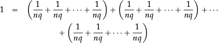
In a similar way, when introducing fractions, we begin by working in some detail with concrete objects and consider “parts of some given whole”. That is, fractions are initially introduced as “parts of a whole”, where the meaning depends on the particular “whole”: in other words, the fractions are “fractions of” something, or operators. Before too long, we need to introduce the fundamental idea that if we take the number “1” to be the whole, and think of fractions as parts of this universal object “1”, we obtain “fractions as numbers”. That is, the unit “1” can be subdivided into n equal parts, each of which is equal to the unit fraction  . This opens the door to a uniform treatment of fractions—including working with fractions that are bigger than 1: the fraction
  can be made by taking m copies of this “unit fractional part” .
Integers were constructed by multiplying (or replicating) the unit to obtain “multiples of the unit 1”:
n = 1 + 1 + 1 + ··· + 1(n terms).
Fractions as numbers arise as
“that part of 1” that emerges when we treat the unit “1” as our “whole”, and apply the fraction as an operator to it.
The unit fraction is obtained by dividing the unit, taking to be “a submultiple of the unit 1”—namely that “part” of which exactly n copies make 1:
1 = + + + ··· + (n terms).
Thus is precisely that number of which 2 identical copies make 1:
1 = + ;
 is precisely that number of which 3 identical copies make 1:
1 = + + ;
 is precisely that number of which 4 identical copies make 1:
1 = + + + ;
and so on.
In the end, this is what every justification for calculation with fractions comes down to.
•The fraction  is defined as above: namely that number of which q copies make 1.
In the spirit of arithmetical division, this is interpreted as the result of dividing the unit 1 into q parts, and then taking one part. In other words, is the answer to the question
•The fraction  is then defined to be p × (that is,
+ + … +
with exactly p terms).
In the spirit of division of given quantities, this can then be proved to be equal to the result of dividing p units (or wholes) into q identical parts and then taking one of the q parts (which is easiest to see by dividing each of the p units into q equal parts [each part being equal to ], and selecting 1 of these parts from each of the p different units, to give p × ). In other words, is defined to be p × , but turns out to be equal to the answer to the question
“p ÷ q = … ?”.
•We know that  is the number of which nq identical copies make 1:

Since there are exactly n × q terms on the RHS, we can bracket them into q successive groups with n terms in each bracket:
There are now q equal brackets on the RHS, so (by the definition of ),
–each bracket must be exactly equal to ;
–and each bracket contains n terms equal to , so each bracket is also equal to n × , which is precisely what we call  .
.
∴ =
An entirely similar argument shows that

so we can replace any given fraction by another fraction equivalent to it by “cancelling”, or by multiplying numerator and denominator by the same integer n.
•Addition and subtraction of fractions needs to be linked to reality by combining fractional parts of a fixed object.
•Any two fractions  and
and  with the same denominator can also be added or subtracted by remembering what they represent—namely a × (that is,
with a terms) and b × (that is,
with b terms), so that
–their sum is
(that is,
–their difference is
(that is,
with a − b terms).
•Any two fractions  and with different denominators can be added or subtracted by first transforming them both into equivalent fractions with the same denominator
so that
–their sum is
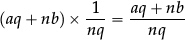
(that is,
with aq + nb terms), and
–their difference is
(that is,
with aq − nb terms).
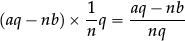
•Division of fraction x by fraction y needs to be linked to reality by discovering that both forms of division give the same answer:
–“How many times does y go into x?” (or “How many times can I subtract y from x?”), and
–“What do we multiply y by to get x?”
•We can formally divide any fraction by one with the same denominator, say , by remembering what they represent—namely a × = and b × = , so that we can switch to the equivalent fraction by multiplying both numerator and denominator by “q” to see that the quotient is  .
.
•To formally divide any fraction by one with a different denominator , we first change them both to equivalent fractions
with the same denominator, and we can then evaluate the quotient by switching to an equivalent quotient by multiplying numerator and denominator by “nq” to see that the quotient is  .
.
•To multiply two unit fractions and we return to their definitions as submultiples of 1, and think about the product
[n terms in the 1st bracket, q terms in the 2nd].
When we multiply out the two brackets we obtain nq equal terms, each equal to

whose sum is 1. But that is precisely the definition of the unit fraction “”.
When we multiply two general fractions and we can write each fraction out as:
and then multiply out the two brackets ‘long hand’ to get
[a terms in 1st bracket, b terms in the 2nd] where the RHS gives rise to exactly ab separate terms, each equal to
1.6.5Fractions and terminating decimalsPupils need exercises that clarify three features of terminating decimals.
The first is to use place value to interpret each decimal as a sum. Just as
375 = 3 × 100 + 7 × 10 + 5,
so place value tells us that 0.375 means precisely the sum
The second is to rewrite the constituent parts (from the separate “places”) with a common power of 10 as denominator (here “1000”) to obtain:
| (*) |

In other words, pupils need to connect the definition of place value (which breaks up the number into a sum of several parts—tenths, hundredths, thousandths, etc.) with the alternative reading of 0.375 as  .
.
The third feature is more subtle, namely to realise precisely which fractions correspond to terminating decimals, and which correspond to endless decimals.
•If a fraction is given with denominator a power of 10, then it is easy to write it as a terminating decimal, in exactly the same way that equation (*) tells us that
| (**) |

•But what do we know about  and
and  that should tell us in advance that the first has a terminating decimal, but the second does not?
The key lies in the previous paragraph (and properties of prime factorisation which were addressed in Section 1.4).
Suppose we are given some unfamiliar fraction.
•The first move is to cancel any common factors between the numerator and the denominator which may mislead us.
For example, we know that the decimal for = 0.5, and so it terminates. But if we were faced instead by  , we might be misled by knowing that the decimal for
  does not terminate. This first move of “cancelling” puts the given fraction into its “standard form”, or “lowest terms”, , where p, q have no common factors (other than 1): HCF(p, q) = 1.
We have seen that a fraction whose denominator is equal to a power of 10 can always be written as a terminating decimal (as in equation (**)). Pupils need to extend this to see that
•if a given fraction can be re-written in a form with denominator equal to a power of 10 (in the same way that =  ),
),
then it will be equal to a terminating decimal.
That is, given a fraction , we need to know when it can be rewritten as an equivalent fraction  which has denominator a power of 10.
If nq is a power of 10 for some multiplier n,
then the denominator q of the given fraction must be a factor of some power of 10.
Now 10 = 2 × 5, so a power of 10, such as 10m = (2 × 5)m, has the form 2m × 5m.
And any factor of 2m × 5m must have the form 2a × 5b for some a, b ⩽ m.
∴ If the fraction has a terminating decimal, then the denominator q must have the form 2a × 5b: that is, a power of 2 times a power of 5.
•Conversely suppose we are given any fraction with denominator q of the form 2a × 5b.
If a ⩾ b, then we can multiply by n = 5a − b to make nq = 2a × 5a = 10a; and if b > a, then we can multiply by n = 2b − a to make nq = 2b × 5b = 10b.
∴ Any fraction with denominator of the form 2a × 5b has a terminating decimal.
Hence whether a given fraction (where p, q have no common factors) has a terminating decimal or not depends entirely on the prime factorisation of the denominator q:
q = 1, 2, 4, 5, 8, 10, 16, 20, 25, 32, …
all lead to terminating decimals, but
q = 3, 6, 7, 9, 11, 12, 13, 14, 15, 17, 18, 19, 21, 22, 23, 24, 26, 27, 28, 29, 30, 31, …
1.6.6Fractions and recurring decimals
Section 1.6.5 shows that:
every fraction , where p, q have no common factors and q is not of the form 2a × 5b has a decimal that does not terminate, and so must go on for ever.
In fact every such fraction has a decimal that “recurs”: that is, its decimal consists of
an initial sequence of digits (which can be of any finite length), followed by a “block of digits” that simply repeats over and over again for ever.
The most familiar examples are
which recurs from the beginning with a repeating block “3” of length 1;
which recurs from the beginning with repeating block “09” of length 2;
which recurs from the 2nd place with repeating block “6” of length 1;
which recurs from the start with repeating block “142857” of length 6.
The converse is also true, in that
every decimal which recurs in this fashion is the decimal of some fraction.
The proofs of these statements are discussed briefly in Section 1.8 below.
1.7.[Subject content: Number p. 6]
–use approximation through rounding to estimate answers and calculate possible resulting errors expressed using inequality notation a < x ⩽ b
In mathematics we calculate with exact “mental objects”. But when mathematics is applied, the numbers often come from the real world. Discrete data from the real world (e.g. small counting numbers) can sometimes be “exact”; but most measurements are reliable only to a certain degree of accuracy. The approximate character of certain measurements is reflected in the “rounding conventions”. When a digit is known to be, or is to be taken as being, just beyond the known or required limits of accuracy, the “rounding conventions” mean that
“a digit of 5 or more is rounded up, and everything else is rounded down”.
Hence a decimal like 37.45293 would be written as
“37.45 to 2 decimal places”, or “37.5 to 1 decimal place”.
Conversely, if we are given a measurement “x = 37.5 to 1 decimal place”, then all we know is that the “true” value of x lies somewhere in an interval: 37.45 ⩽ x < 37.55. (The inequality given in the official requirement listed at the start of 1.7 should probably have been written as “a ⩽ x < b” to fit in with this convention.)
If the initial data is only known to a certain degree of accuracy, then any calculation with that data is approximate from the outset. Even when our data and our calculations are “theoretically exact”, approximations may arise when exact terms (such as “ sin 45°” or “”) are “evaluated” at some point using a decimal approximation. All approximations affect the accuracy of the final result; so pupils need to understand how potential errors “accumulate” as a result of calculation, so that they can tell exactly how inaccurate the final result could be.
When adding or subtracting approximate numbers, the errors in the data add up. Given two lengths of 2.15cm and 1.75cm—each correct to within 0.05cm—their calculated difference of 0.40cm is only correct to within 0.1cm, so could actually be as low as 0.30cm or as high as 0.50cm. And if we were to add four lengths, each of which was accurate to within 0.05cm, then the result would only be accurate to within 0.2cm either way (so we would only know that the answer lies in an interval of length 0.4cm).
When multiplying or dividing the story is a more complicated. For example, the area of a rectangle whose dimensions are given as “15cm by 12cm”, where each measurement is accurate to within an error of 0.1cm, is equal to 15 × 12cm2, or 180cm2, but only to within 2.7cm2. And if we know that a rectangle has area 180cm2 accurate to within 5cm2, and that its length is 20cm accurate to within 0.1cm, then its width may be as small as small as (175 ÷ 20.1)cm ≈ 8.7cm (to 1 d.p.), or as large as (185 ÷ 19.9)cm ≈ 9.3cm (to 1 d.p.).
The art of making estimates, or approximate calculations, is more subtle than is often thought. It depends on:
•robust fluency in exact calculation, together with a “feeling for calculation” that is willing to think flexibly about the effect of any errors,
•a willingness to change global units intelligently (replacing the given units by larger or smaller “blocks” so as to make the eventual calculation more manageable), and
•an ability to make sensible local approximations (to find the approximate size of one of these new ‘blocks’ and to estimate the number of “blocks”).
Consider first approximating an exact arithmetical calculation, such as 35941 × 273.
•We need the kind of flexibility that can think of this as 35941 “blocks” of 273, and combine this with a clear understanding of how the exact calculation would proceed using the given units—with 35941 copies of a collection of size 273.
•Instead of 35941 blocks (each of size 273) we then may see the advantage of interpreting the number of blocks as “slightly more than 33 thousand”, and compensate the block size of 273 by thinking of it as “slightly less than 3 hundreds”.
•This then suggests that the required answer is “approximately 100 hundred thousands”, or 10 million.
By increasing one factor in the product and decreasing the other we managed to produce an answer that is fairly close to the actual value (9 811 893) of the product. But the method used gave us no clue as to whether we had overestimated or underestimated, or what our maximum error might be. To get such assurance we would have to approximate consistently—perhaps to work out
first an overestimate such as 36000 × 300 = 10800000,
then an underestimate such as 35000 × 250 = 8750000.
Similarly, in seeking to estimate the size of a large crowd, one may divide the whole into a number of blocks of more-or-less the same size, count (or estimate) the number in a given section of the crowd relatively accurately (for example, by counting the number of rows and the number in each row), and then multiply the answer by the number of blocks. A striking historical example of this approach to estimation occurs in Herodotus, The Histories, Book 7:
“As nobody has left a record, I cannot state the precise numbers provided by each separate nation [towards the Persian army that Xerxes was leading against the Greeks in around 480BC], but the grand total, excluding the naval contingent, turned out to be 1 700 000. The counting was done by first packing ten thousand men as close together as they could stand and then drawing a circle around them on the ground; they were then dismissed and a fence, about navel-high, was constructed round the circle; finally the other troops were marched into the area thus enclosed and dismissed in their turn, until the whole army had been counted.”
1.8.[Subject content: Number p. 6]
–appreciate the infinite nature of the sets of integers, real and rational numbers.
There is an awkward clash between the precise, procedural language which is appropriate for specifying the ideas and processes of a school curriculum and this highly unusual and rather woolly “requirement”. Indeed, it remains unclear how it survived the extended editing process.
The underlying idea would be fine as part of an internal curriculum—for in some sense, the whole of elementary mathematics is the story of “how we tame infinity”. But to include such a requirement in a national curriculum (especially in such a curiously worded form) runs the risk that some examiner may decide that they are obliged to invent some way of “assessing” each year whether it has been addressed!
1.8.1Mathematics begins when we move beyond the particular to the general. Every culture develops some way of referring to the size of small collections of objects (one, two, three, …), and to the ordering of its objects (first, second, third, …). They either develop some semi-systematic counting process or adapt that of some neighbouring culture for their own use. Some cultures go further and invent an “arithmetic” based on their counting process; but this is almost always done without worrying whether their form of counting could “go on for ever”.
For example, the numeration system of the Egyptians, and that of the Babylonians, were both semi-systematic. But both were restricted by the need to invent specific new symbols each time they wanted to refer to larger numbers; so it is unclear whether they appreciated “the infinite nature of the set of integers”. In contrast, there is something truly remarkable about the ease with which our Hindu-Arabic numeral system combines the ten digits 0-9 and the idea of “place value” to convey the idea that counting
1, 2, 3, 4, 5, 6, 7, 8, 9, 10, 11, 12, 13, 14, 15, 16, 17, 18, 19, 20, 21, 22, … , 98, 99, 100, 101, …
can continue for ever, even though we soon run out of linguistic ways of “naming” the numbers whose numerals we can all write down so easily.
Despite their mathematical sophistication, the Greeks had no such systematic notation—a lack which may have forced them to develop their astonishingly modern approach to handling infinity and infinite processes. But it also meant that Archimedes had to go to considerable lengths to demonstrate (in his little book, The Sand Reckoner) that “the number of grains of sand in the universe is finite”. This he did by repeatedly changing units in order to estimate a finite upper bound (around 8 × 1063) based on constructing a large power of a number called (in Greek) a “myriad myriad”—in much the same way as Herodotus reported (Section 1.7 above) that the Persians counted the number of soldiers in Xerxes’ army as a multiple of ten thousand.
Our numeral system avoids the inevitable finiteness of number names, and focuses instead on a numeral system based on place value, which allows us to write numbers without giving them names. It then seems clear that, using only the digits 0–9, our written numerals for counting numbers could go on for ever. (The truth is more delicate. In our numeral system we “deduce” the endlessness of the sequence of counting numbers by first assuming that the sequence of possible “places”—the units, tens, hundred, thousands, etc.—goes on for ever! However, this is unlikely to disturb anyone.)
In some sense, that is all there is to it. The counting numbers are the same as the positive integers, so the integers—both positive and negative—are also infinite (that is, “more than just finite”). The integers are precisely the “rational numbers with denominator 1”, so the set of rational numbers is even bigger—and hence infinite. And the real numbers include all the rational numbers—so the set of all real numbers is also infinite.
1.8.2Sequences: What else is there to be said at secondary level? Endless sequences use the counting numbers to label the successive terms of a sequence. The squares, the cubes, the powers of 2—all go on for ever, and all get larger and larger without bound (though some “grow” faster than others):
02 = 0, 12 = 1, 22 = 4, 32 = 9, 42 = 16, … , n2, … ;
03 = 0, 13 = 1, 23 = 8, 33 = 27, 43 = 64, … , n3, … ;
20 = 1, 21 = 2, 22 = 4, 23 = 8, 24 = 16, … , 2n, … .
Some sequences eventually stop. Others go on for ever, with one such term for each positive integer n. It is hard to see that there is much to make a fuss about.
However, there are two clear candidates at this level, which show that indeed there is indeed something interesting here, to which one might draw attention—at least for suitable groups of pupils. The first concerns prime numbers; the second concerns the way we can be sure that fractions are precisely the real numbers whose decimals either terminate or recur.
1.8.3Prime numbers: Prime numbers are the multiplicative building blocks for integers.
There are 4 prime numbers up to 10; 25 up to 100; and 168 up to 1000.
That is: prime numbers make up 40% of integers up to 10; 25% up to 100; 16.8% up to 1000.
It is thus apparent that prime numbers seem to be “thinning out” as one goes up. So one might ask:
Do the prime numbers eventually “peter out”? Or do they go on for ever?
There is no indication that anyone considered such a question before the Greeks (4th century BC), who proved that
“the prime numbers are more than any assigned multitude”.
That is, that the prime numbers go on for ever. Euclid’s original proof is highly memorable and has impressed many a young mind—but it is often misrepresented. We give it here in a form that is both close to the original, and in the spirit of modern constructive mathematics.
We know a few prime numbers, so we can clearly pick one to start with—say p1. (We could choose p1 = 2, but we do not have to.)
N1 = p1 + 1
to be “1 more than the product of all the primes in our list so far”.
∴ p1 is not a factor of N1 (since it leaves remainder = 1); so the smallest prime factor p2 of N1 is a new prime number.
Then set
N2 = p1 × p2 + 1
to be “1 more than the product of all the primes in our list so far”.
∴ Neither p1 nor p2 is a factor of N2 (since both leave remainder = 1); so the smallest prime factor p3 of N2 is a new prime number.
Then set
N3 = p1 × p2 × p3 + 1
to be “1 more than the product of all primes in our list so far”.
∴ None of p1, p2, p3 is a factor of N3 (since all leave remainder = 1); so the smallest prime factor p4 of N3 is a new prime number.
And so it goes on, for ever. QED
That is, once the list gets started, no matter how many primes we have listed so far, we have a bomb-proof way of finding a new prime.
Suppose we start with p1 = 2, then N1 = 3 is prime, so p2 = 3;
then N2 = 7 is prime, so p3 = 7;
then N3 = 43 is prime, so p4 = 43.
It is important not to stop at this point, but to complete the next three stages in order to understand how the process really works.
Work out
N4 = 2 × 3 × 7 × 43 + 1,
and hence find its smallest prime factor p5 = … .
Then work out
N5 = 2 × 3 × 7 × 43 × p5 + 1,
and hence find its smallest prime factor p6 = … .
Then work out
N6 = 2 × 3 × 7 × 43 × p5 × p6 + 1,
and hence find its smallest prime factor p7.
It is also worth starting with various different “initial primes” p1 to see how this affects the sequence which is generated each time.
Those who took up our earlier suggestion (Section 1.3) of challenging pupils to
“Find a prime number which is one less than a square. Find another. And another.”
might also like to use the similar-sounding, but actually very different challenge:
“(a) Find a prime number which is one more than a square
(b) Find another such prime. And another.”
If one tries this, then it quickly becomes clear that, except for the very first such prime 12 + 1 = 2, one can restrict to looking for odd primes, and these must be “one more than an even square”. Among the list of numbers that are “one more than an even square”,
22 + 1, 82 + 1, 122 + 1, 182 + 1, 222 + 1, 282 + 1, …
If we eliminate these multiples of 5, we are left with a long list of candidate primes, starting:
(2,) 5, 17, 37, 101, 197, 257, 401, 577, 677, 901, …
Almost all of these 11 “candidate primes” turn out to be genuine primes (only one of those listed is not). This raises the question:
Are there infinitely many prime numbers of the form “n2 + 1”?
Or does the list eventually peter out?
This is perhaps the simplest question one can pose at this level to which the answer is not yet known.
1.8.4Recurring decimals:One other place where infinity features at Key Stage 3 and needs to be handled properly is the way the normal division process is extended to compute recurring decimals for fractions. We have seen that when we divide an integer p by another integer q, the process terminates precisely when the fraction is equivalent to a decimal fraction (one with denominator 10n for some n)—as with

or

and that this occurs whenever the fully simplified fraction has a denominator of the form 2a × 5b.
In all other cases, the division process continues indefinitely. For example, when one carries out the division for  , the output seems to recur: 0.14285714… . All too often pupils are left with the impression that
the output to the division process “recurs” because it seems to recur.
This is like believing that the “leading digits” of the sequence of powers of 2 recur because they look as though they recur:
2, 4, 8, 1, 3, 6, 1, 2, 5, 1; 2, 4, 8, 1, … .
The fact that the division of p by q recurs follows not from the apparent output, but from the pattern of remainders.
•The decimal for terminates precisely when at some point we obtain a remainder of 0.
•So if the decimal does not terminate, then the only possible remainders are
1, 2, 3, … , q − 1.
Hence, within at most q steps, we will always get a remainder r that we have seen before; and this remainder r becomes 10r in the next decimal place as it did on the first occurrence of the remainder r, so from then on the process simply repeats whatever happened after the previous occurrence of the remainder r.
For example, when calculating the decimal for we divide 7 into 1.000000… .
•Forget about the output, or the “answer”, and concentrate on the remainders.
•The process begins with a remainder of “1”, then “3”, then “2”, then “6”, then “4” then “5”, then “1” (the first repeat)—which becomes “10” in the next column, as it did at the first stage when the initial “1” became “10 tenths”.
•The process must then repeat from here on (giving the answer
0.14285714285714… ,
with the block “142857” repeating for ever).
The converse claim—namely that
every number x whose decimal recurs is the decimal of some fraction
can be appreciated at this level (say Year 9 or Year 10) via the procedure for turning any such decimal back into a fraction. For example:
Suppose x = 0.37255555… (for ever)
Then 10x = 3.72555555… (for ever)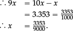
Suppose x = 0.72525252525… (for ever)
Then 100x = 72.5252525252… (for ever)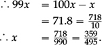
1.9.[Subject content: Ratio, proportion and rates of change p. 7]
–change freely between related standard units (for example time, length, area, volume/capacity, mass)
–use scale factors, scale diagrams and maps
–express one quantity as a fraction of another, where the fraction is less than 1 and [where the fraction is] greater than 1
–use ratio notation, including reduction to simplest form
–divide a given quantity into two parts in a given part:part or part:whole ratio; express the division of a quantity into two parts as a ratio
–understand that a multiplicative relationship between two quantities can be expressed as a ratio or a fraction
–relate the language of ratios and the associated calculations to the arithmetic of fractions and to linear functions
–solve problems involving percentage change, including: percentage increase, decrease and original value problems and simple interest in financial mathematics
–solve problems involving direct and inverse proportion, including graphical and algebraic representations
–use compound units such as speed, unit pricing and density to solve problems
1.9.1This is a mixed bag of requirements linked to multiplication, ratio and proportion, and scaling—and hence, ultimately to the application of fractions.
•The first two listed requirements (the ability to switch “between related units”, and to work with “scale factors, scale diagrams and maps”) clearly involve “multiplying factors” and an application of ratios.
•We have already noted the relative neglect of compound units. So the last listed requirement in 1.9 should be interpreted in the light of comments already made in Section 1.1 above and in Part II, Section 1.2.
•Percentage and percentage change has already arisen in 1.6, but reappears here for good reason.
•The requirements for pupils to “express one quantity as a fraction of another” and to “divide a given quantity into two parts” underline the connections between the work required here and work involving fractions (see Sections 1.6.1–1.6.3 above).
1.9.2We repeat and expand some of the ideas touched upon in Part II, Section 2.2.1. Elementary mathematics comes into its own (and needs to be seriously taught!) as soon as we take the step from addition to multiplication. Ratios are the quintessential “multiplicative relations”, and work with ratios links naturally to work with fractions.
All that is needed to generate a ratio is a single class of comparable magnitudes—that is, a class of magnitudes
•where any two given entities can be “compared”, so that we can decide which is the larger, and
•where one can also subtract the smaller from the larger, with the “difference” being another entity from the same class (as, for example, with line segments).
That is, one needs to be able to implement a version of the Euclidean algorithm.
The simplest example of a class of “comparable magnitudes” is the set of positive real numbers. In the context of ratios, real numbers normally arise as the set of numerical measures of some set of objects (relative to some chosen unit). Such numerical ratios are easy to handle (with the class of objects being replaced by their measures); but ratios also arise naturally in mathematics between comparable entities (such as line segments, or 2D shapes) without turning everything into numbers by ‘measuring’.
For example, 3cm and 2cm are in the ratio “3 : 2”. But we also have the same ratio between the two line segments, say AB and CD, that were measured as being of lengths 3cm and 2cm. Even if we do not know their exact lengths, there is often a natural way to be sure that “half of the second segment fits exactly three times into the first segment”. For example, if we draw a circle with centre O passing through the point X, extend the radius XO to meet the circle again at Y, and construct the mid-point M of the segment OY, then we can be sure (without measuring) that
XM : XO = 3 : 2.
1.9.3The rest of our comments in this section revisit and extend our previous remarks in Part II, Section 2.2.1. What follows explores further the background to ratio and proportion, which is the key idea that underlies most of the (rather vaguely worded) requirements listed at the start of Section 1.9. We repeat our earlier comment: this outline is intended for teachers, and is not a teaching sequence for pupils.
The word proportion has a colloquial usage, which is unfortunately copied in many mathematics texts and classrooms. People speak about “a proportion of the class”, meaning exactly the same as “a fraction of the class”. This has nothing to do with mathematical “proportion”. Sloppy language is neither helpful nor harmless: it confuses pupils, teachers, textbook authors, and examiners alike. In general, technical words are best used correctly and with care in the mathematics classroom (as is normal in many other countries). Because the underlying mathematics may not be second nature, it seems simplest to repeat the basic framework from Part II, Section 2.2.1, while adding a little more detail.
Given the notion of a class of comparable magnitudes, or quantities, a (mathematical) proportion arises when two different classes of entities are linked in a special (but very common) way. For example, suppose that one class consists of
“quantities of petrol”
and the other class consists of
| “amounts of money in £”. |
If 1 litre of petrol | costs £1.50, |
then we expect 2 litres | to cost £3 (= 2 × £1.50) |
That is, for any two purchases from the same outlet at the same time, the quantities purchased (in litres)
are in the same ratio as
| the amounts paid (in £). |
If I buy a litres of petrol | and pay £c, |
and you buy b litres of petrol | and pay £d, |
then the ratio a : b | is equal to the ratio c : d. |
The equality
a : b = c : d
is what we call a proportion.
Note that since a, b, c, d are magnitudes, with a, b of one kind and c, d of another kind, then “a : b” is a perfectly well-defined ratio; but “a : c” makes no sense, because a and c are not “comparable magnitudes”. One can have a ratio a : b between two quantities of petrol both measured in litres (or a ratio c : d between two amounts of money—both measured in £); but one cannot have a ratio between a quantity of fluid and an amount of money.
However, something miraculous occurs if we replace the different quantities and amounts by their numerical measures. The equality of ratios
a : b = c : d
can then be written as an equation between fractions, which can be treated purely algebraically. That is, if we replace each ratio by the quotient of the corresponding measures we get an equality of quotients, or fractions:
| (*) |

The two quotients in equation (*) are always equal, but can take any positive value. For example, we could buy
b = 2a litres of petrolandpay d = 2c pounds,
and the quotients would both take the value . Or we could buy
b = a litres of petrolandpay d = c pounds,
and the quotients would both take the value 2.
The equation (*) between fractions can be treated purely numerically (or algebraically) and can be rearranged to give

This equation looks very similar to equation (*), but it is completely different. The two sides do not represent ratios, but specify the constant of proportionality (relative to the two chosen units: litres and pounds (£)). That is, once we choose units and give numerical values a and c to the basic pair of corresponding magnitudes—one from one class and one from the other
alitres ![]() cost £c
cost £c
the value of the quotient  is a constant: that is, it is the same as the value of the corresponding quotient
  for any other pair of corresponding magnitudes b, d (one from one class and one from the other). The purely numerical quotient can now be interpreted as the “multiplying factor” that links the two classes of related magnitudes.
This is the simplest, and perhaps the most valuable, application of school mathematics—to life, to science and to mathematics itself. It applies whenever two quantities are related so that if one quantity doubles, or triples, so does the other: that is, where the numerical measures a, c or b, d of the two quantities have a constant ratio. Two quantities that vary in such a way as to preserve a constant ratio between their values are said to be “in proportion”.
The fact that “ is a constant” means that the number lines corresponding to the two families of measures “line up” in such a way that one scale is simply a multiple (× ) of the other:
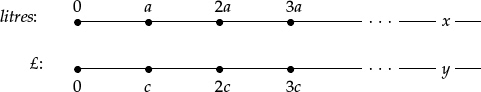
If we imagine a linked pair (x, y) of unknown variables—where
xlitres ![]() cost £y
cost £y
then these linked variables are related by the linear equation

Eventually (in late Key Stage 3 or Key Stage 4) one may want as many pupils as possible to appreciate this global picture, and to be able to
“formulate proportional relations algebraically”
as is required in the quote at the start of Section 2.2.1 in Part II. However, this is unnecessary, and probably inappropriate for beginners, who first need to learn how to solve the various standard problems involving proportion.
Any particular proportion problem that pupils may be required to solve is likely to involve just two pairs (a, c) and (b, d),
where a and b come from one class of magnitudes,
and c and d come from the other class.
In a typical proportion problem, three of the four values are known and the fourth is “to be found”. This explains why the approach to solving this kind of problem is referred to in old texts as “the rule of three”. Hence one pair is completely known, and we take this as our “base”, or reference pair
a litres ![]() cost £c
cost £c
One of the other two values is to be found. So the four ingredients can be thought of as the corners of a rectangular array, where three of the values are known and the fourth is to be calculated, so we either have the unknown value in the bottom right corner:
Ifa litres ![]() cost £c
cost £c
thenb litres ![]() cost £??
cost £??
or the missing value may be located bottom left:
Ifa litres ![]() cost £c
cost £c
then?? litres ![]() cost £d
cost £d
This standard way of representing the four pieces of information in a proportion—with three known values and one generally unknown—is referred to here as the rectangular template for displaying proportion problems.
To repeat the earlier derivation, if we know the corresponding values a and c in our “reference pair”
a ![]() c
c
then two unknown amounts x and y, which correspond to each other, provide the third and fourth vertices of our “rectangular template”
x ![]() y
y
and so satisfy
x : a = y : c
If the two magnitudes of the first kind x, a, and the two magnitudes of the second kind y, c are replaced by their measures, then the proportion can be written as

and this can be rearranged to express the relationship between the two unknown values x and y as

with multiplying factor . If we are given the value of x, we can calculate the value of

and if we are given the value of y, then we can calculate the value of

For example:
if a = £100 | is worth the same as | c = $150 |
then
x = £200 | will be worth exactly | y = |
And
if a = 1kg | is the same as | c = 2.205lbs |
then
x = | is the same as | y = 5lbs. |
 × y = … kg
Earlier we showed how the “number lines” corresponding to the two families of magnitudes in a proportion problem can be lined up to form what is sometimes called a “double number line”. We have since seen how the simpler “rectangular template” picks out two data points (a and b) on the first number line, and two points (c and d) on the second number line, and have suggested that this is sufficient for the beginner to solve problems. (To link the two representations one has to imagine that the double number lines run vertically, with a and b chosen from the left hand line and c and d chosen from the right hand line.)
We typically know one pair of corresponding values, such as that
£100 | is worth | $150; |
and we want to know either:
“If I have £x = £768 |
| how many $y can I expect in exchange?” |
or
“How many £x should I |
| expect in exchange for y = $1152?”. |
Pupils who become sufficiently confident may solve the first kind of proportion question directly—and in one of two ways:
(i) | extract the ratio
(150 × |
(ii) | identify the constant of proportionality
( |
 in the above example), and apply it to the third known quantity c of the other kind, to find the unknown required value
 in our example) derived from two known corresponding quantities of different kinds, and apply it to the third known quantity b to find the unknown value
 × 768 = … in the above example).
However, for most students, the unitary method provides an essential stepping stone en route to this general method—a stepping stone which one can return to in any setting to re-explain, or to reinforce, the logic of the general method.
Given three of the four relevant values,
instead of using one of the two “magic multipliers” ( or ) immediately, we use the two known corresponding values (one of each kind)—here £100 and $150—to calculate:
•first that
£1 (the unit)corresponds to$  = $1.50
•then to multiply the answer ($1.50) by 768 to get the number of $
£768 = 768 × £1corresponds to768 × $1.50 = ….
Thus
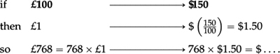
We noted in Part II Section 2.1.1 that elementary algebra has its roots in structural arithmetic—the art of numerical calculation which exploits structure rather than brute force.
•At its simplest, this appeal to “structure” may go no further than to use place value—as in
73 + 48 + 27 = (73 + 27) + 48,
or
17.18 + 7460 + 22.82 = (17.18 + 22.82) + 7460.
•This grows into an awareness of the algebraic structure lurking beneath the surface of many numerical or symbolical expressions—as in
3 × 17 + 7 × 17 = (3 + 7)× 17,
or
or
16 × 17 − 3 × 34 = (16 − 6) × 17.
•Eventually this instinct for “tidying up” applies the underlying algebraic rules in a way that allows us to simplify all manner of algebraic expressions—starting with the simplest examples, such as
6(a − b) + 3(2b − a) = … .
But before this third stage, pupils must first internalise these algebraic rules by applying them to simplify numerical expressions, and then learn to see symbols as “placeholders for numbers” and to calculate with symbols in this spirit.
It is not easy to illustrate what we in England need to do differently with algebra at age 11–14. The complaints of those who teach the top 20% at the start of A level mathematics at age 16 are clear and consistent: these students—who are the most successful products of Key Stage 3 and Key Stage 4—struggle with fractions, and with the simple algebra they need for beginning A level. Other pupils are even more ill-served by the current approach to algebra up to age 16, where this key topic is either ignored, or treated far too superficially. We need to lay much stronger foundations in algebra for all pupils (even if some will inevitably go further than others).
The more focused demands of the new Key Stage 4 programme of study could provide a useful indication of what needs to be done—provided these demands are understood, and are taught with a view to mastery (rather than as mindless rules). Another useful pointer as to what needs attention may be found in the released items20 from TIMSS 2011, which compared achievement in around 50 countries. English Year 9 pupils do tolerably well as long as they only need to use their common sense (e.g. “pattern spotting”). But once their performance depends on technique (i.e. something that has to be taught), the results are less encouraging. We saw in Part II (examples 1.4A–1.4K) how the bulk of Year 9 pupils in England struggle with simple problems involving fractions and decimals. In Sections 2.4, 2.5, and 2.7 below we include a selection of items intended to support the assertion that schools also need to re-consider how they approach algebra at Key Stage 3. We have again avoided making comparisons with countries from the Far East, and instead compare the results of pupils in England with those from Russia, from Hungary, from the USA, and from Australia.
2.3.[Subject content: Algebra p. 6]
–use and interpret algebraic notation, including
ab in place of a × b
3y in place of y + y + y and 3 × y
a2 in place of a × a, a3 in place of a × a × a, a2b in place of a × a × b
 in place of a ÷ b
coefficients written as fractions rather than as decimals
brackets
It would be hard to overstate the extent to which the algebraic notation summarised in these six bullet points makes elementary mathematics accessible to ordinary people.
The importance of notation should be clear if one considers the impact of our notation for writing integers and decimals in base 10. This was proposed in 1585 by the Dutchman Simon Stevin in his little book Die Thiende. Stevin’s original notation was slightly unwieldy, but it soon evolved into the astonishingly compressed form that we use today, where a single succession of digits (and a decimal point) captures everything about a number, and does so in a way that allows routine calculation in a form that everyone can master. This notation was later extended by adopting our way of writing fractions or quotients (see the fourth bullet point above), and surds.
Our algebraic notation then emerged in almost modern form in Descartes’ book on Geometry in 1637. This had an even greater impact. Before that time, even the best mathematicians struggled to express general calculations using symbols. Yet within 40 years, Descartes’ new symbolism had revolutionised mathematics, allowing Newton and Leibniz to invent what we now call “the calculus”. And within another 100 years, the language of algebra had been streamlined further by Euler into a form that made its potential power available to everyone.
But for ordinary mortals to access this power, the conventions summarised at the start of 2.3 have to be learned and respected. It seems not to be generally understood why these conventions make such a difference; but there is nothing difficult here, and beginners need to be absolutely clear that the conventions are not optional.
The whole purpose of algebraic notation as summarised above is
•to write algebraic expressions in a compact form, that can be apprehended at a glance, and
•to do so in a way that reflects the rules for priority of operations.
The genius of the Descartes-Euler conventions lies in the way they ensure that:
•Multiplication and division hold together tightly, allowing products (such as “3ab” or “5a2b”) to be spatially compressed, so that the eye and the brain perceive them as a single “term”.
•In the same spirit, fractions—whether as coefficients, or as terms within the overall expression—must be written with a horizontal bar (as a, never in the misleading form “1/2a”); and decimals are best avoided whenever possible, since they undermine the goal of holding terms together compactly.
•Addition and subtraction link separate multiplicative “terms”, but do so more loosely, so that the visual impression at a glance reflects the priority of operations.
The result is that the eye and brain can learn to read an algebraic expression at a glance in much the same way as place value allows one to grasp the meaning of numbers. But first one has to learn to routinely and reliably translate mildly complicated combinations into this new algebraic script. Thus one would like almost all pupils to be able to grasp the meaning of the simplest expression, such as “xy + 1”—especially if all they had to do was to choose between four mostly dodgy options.
2.3A What does xy + 1 mean?
A add 1 to y, then multiply by x | B multiply x and y by 1 |
C add x to y, then add 1 | D multiply x by y, then add 1 |
2.3A Russia 89%,USA 80%,Hungary 73%,England 72%,Australia 71%
Given the importance of algebra in elementary mathematics, we really do need to think how to get understanding at this most basic level up around 90%. So in Section 2.5 we stray from our usual “higher viewpoint” and risk a few specific suggestions to encourage schools to consider what we might be currently omitting.
One important point is obscured by the simple examples used in the requirements listed at the start of the current Section 2.3—namely that the ingredient constructions and conventions are often combined. Hence in a typical “sum” the terms being added may themselves already be compound expressions (as in “(3x − 6y + 4) + (5y − 2x − 3)”), and in a typical “square” the expression being squared may be a compound expression (as in “(3x − 6y + 4)2”). Too often we stop short of adding this extra layer of complexity. In the short term, nothing may be lost; but such “layered complexity”, or variation, is an integral part of the new algebraic language, which pupils need to get used to.
2.4.[Subject content: Algebra p. 6]
–substitute numerical values into formulae and expressions, including scientific formulae
–understand and use standard mathematical formulae; rearrange formulae to change the subject
–understand and use the concepts and vocabulary of expressions, equations, inequalities, terms and factors
–simplify and manipulate algebraic expressions to maintain equivalence by:
–collecting like terms
–multiplying out a single term over a bracket
–taking out common factors
–expanding products of two or more binomials
Section 2.4.1 addresses the content of these four requirements by providing some initial food for thought from TIMSS 2011, a study which compared the performance of Year 9 pupils in around 50 countries.
Section 2.4.3 is long and expands on our earlier remark that “Elementary algebra copies the structure of arithmetic (that is, the four rules, together with the commutative laws, the associative laws, and the distributive law), and applies it to a new mixed universe of symbols (or letters) and numbers.”
Section 2.4.2 is relatively short, and refers loosely to some of the ideas from 2.4.3, so should perhaps follow it. But that would risk the basic message of 2.4.2 being obscured by the preceding detail. Since this message is simple and important, we present it before the details in Section 2.4.3.
2.4.1We begin with six tasks taken from TIMSS 2011. The first three are simple exercises involving substitution, and so are directly relevant to the first listed requirement in 2.4. The last three—two of which are again simple exercises—are relevant to the second, third and fourth requirements (and especially the fourth).
2.4A y = a +  . a = 8, b = 6, and c = 2. What is the value of y?
A 7B 10C 11D 14
2.4B k = 7 and m = 10. What is the value of P when P =  km?
km?
2.4C Use the formula
to find the value of y when t = 9.
2.4D Which of the following is equal to 3p2 + 2p + 2p2 + p?
A 8pB 8p2C 5p2 + 3pD 7p2 + p
2.4E Which expression is equal to 4(3 + x)?
A 12 + xB 7 + xC 12 + 4xD 12x
2.4F Simplify the expression

Show your work.
Once the conventions of elementary algebra are understood, substituting values should be entirely routine. Hence 2.4A, 2.4B, and 2.4C should be exercises in simple arithmetic—where we should expect a high level of success.
2.4D and 2.4E go beyond mere arithmetic, but remain the very simplest kind of algebraic exercises; so one should again expect success rates to be high.
The actual results for 2.4A, 2.4B, and 2.4C (see below) suggest either: that Year 9 arithmetic is weak; or that the conventions of elementary algebra are often not understood at this level. The results for 2.4D and 2.4E (multiple-choice questions with just four rather crude options) suggest that pupils’ grasp of the basic algebraic conventions remains painfully weak.
2.4F is more searching. It is the simplest imaginable example of genuine algebraic simplification involving fractions (as opposed to an introductory textbook exercise); but it requires pupils to have understood that adding fractions requires one to reduce to a common denominator. This idea has to be applied in a mildly algebraic context—but it is hard to imagine what other standard principle might be elicited by the instruction to “simplify” such an expression. The results suggest that schools need to reflect on their current approach to the arithmetic of fractions and to elementary algebra.
2.4A Russia 91%,USA 81%,Hungary 81%,England 73%,Australia 71%
2.4B Russia 83%,USA 70%,Australia 46%,Hungary 46%,England 40%
2.4C Russia 80%,USA 55%,Hungary 51%,Australia 47%,England 45%
2.4D Russia 81%,Hungary 63%,USA 58%,Australia 56%,England 47%
2.4E Russia 81%,Hungary 57%,USA 53%,England 41%,Australia 40%
2.4F Russia 35%,Hungary 34%,USA 19%,Australia 14%,England 9%
2.4.2“Substituting values into formulae and expressions” to highlight letters as placeholders for numbers The requirement to “substitute numerical values into formulae and expressions” draws attention to a basic characteristic of algebra which deserves more attention.
•In an equation the letters are constrained, so can only take particular (as yet unknown) values. So we are not free to “substitute arbitrary numerical values” for the unknown.
•A formula is essentially no different from an equation with two or more variables, in that it expresses the way one variable depends on, and is determined by, others. So we are only free to “substitute numerical values” for certain variables—and this then determines the value of some other quantity which depends on them.
•In contrast, the letters and numbers in an algebraic expression are only required to satisfy the rules of arithmetic (or of algebra), so the letters can be replaced by any numbers whatsoever, provided all occurrences of the same letter are given the same value.
Many pupils never grasp these facts, and blindly move letters around without ever realising that they are little more than “placeholders for numbers”. The examples 2.4A, 2.4B, and 2.4C reinforce the impression that pupils need more varied, carefully designed experiences of “substituting given numerical values” for the letters in “formulae and expressions”, so that they internalise the idea that each letter in an expression can be given any value.
The act of substituting and evaluating also provides opportunities
•to exercise mental arithmetic, and
•to check in a numerical context (and if necessary to correct) the way algebraic notation is understood—including brackets, the correct reading and evaluation of expressions involving exponents, the priority of operations, juxtaposition as multiplication, and the fraction bar as division.
Moreover, evaluating expressions in this way can begin to convey the idea that
•each choice of inputs gives rise to a single determined output value for the expression.
That is, that such expressions provide the simplest examples of what we will later call a function (of is component variables).
2.4.3What is elementary algebra?
We saw in 2.3 how the Descartes-Euler notation for elementary algebra helps us to make sense of compound expressions as being made up from their atomic parts, which we call “terms”. There is no strict definition of what counts as a “term”, but it tends to refer to one of the products, or brackets, which are combined to make up the whole expression. For example, where an integer such as 35 can be written as a product of two integers (35 = 5 × 7), the 5 and 7 are called factors of 35. Similarly, when a compound expression (such as x2 + 5x + 6) can be written as a product of two or more brackets (x2 + 5x + 6 = (x + 2)(x + 3)), each of the brackets on the RHS is a factor of the original expression. In the expanded form, “x2”, “5x”, and “6” would be seen as separate terms; but in the factorised form, the separate brackets “(x + 2)” and “(x + 3)” might be referred to as constituent terms.
This new domain of elementary “algebra” has several distinct sub-domains, each of which sheds a slightly different light on the subject. Some of these subdomains are more natural starting points for beginners than others. The four most obvious subdomains—in approximate order of sophistication—are formulae, equations (and inequalities), expressions, and identities.
•Formulae. Here letters are used in place of familiar entities (e.g. A = l × b for the area A of a rectangle of length l and breadth b; or C = 2πr for the circumference C of a circle of radius r). In each such formula, the letters can take different values. The simplest formulae are a bit like the simplest calculations that we meet at Key Stages 1 and 2, in that they tell us how the value of one entity can be calculated once we know the values of certain others. For a rectangle, A = l × b tells us that the area of a rectangle (measured in square units) is given by multiplying the length and the breadth: the entities l and b can take any value ⩾ 0, and the value of A is then determined.
At Key Stage 3 it is important to stress that, even though symbols (like l and b) are often chosen so that the letters reminds us of what they represent, the symbols are not a shorthand for the concepts “length” and “breadth”, but stand for numbers. Hence b stands for “the number of units in the breadth” rather than for the breadth itself, and the r in 2πr stands for “the length in units of the radius” (see Sections 2.4.1 above and Part II, Section 2.1.3).
[There may be a clash here with the way variables are used in science. In mathematics letters stand for pure numbers. But science teachers sometimes use letters to stand for quantities—including their units: so a letter may be used to stand for a length “3cm”, rather than just for the number of centimetres—namely “3”.]
•Equations (and inequalities). The first equations one meets involve a single letter (often denoted by “x”). This letter is usually referred to as the “unknown”—because an equation can be interpreted as an arithmetical constraint which some “unknown number x” has to satisfy. An equation can then be transformed using the rules of algebra to try to unmask this previously “unknown number”. For example, the problem:
“I’m thinking of a number.
When I double it and add 3 the result is 15.
What is my number?”
can be formulated by saying:
Let the unknown number be “x”.
Then x must satisfy the equation 2x + 3 = 15.
Once the equation has been set up, the secret is to forget where it came from and to transform the equation according to the laws of arithmetic (or the laws of algebra) in order to recover what information we can about “x”: for example,
adding “−3” to both sides we get 2x = 12;
then dividing both sides by 2 we get x = 6.
These “transformations of an equation” set the scene for the way the “=” sign will be routinely handled when pupils work with expressions and identities.
Later we meet equations involving the square or the cube of the “unknown”, or equations involving more than one “unknown”. For example, suppose we are asked:
“How can I transfer exactly 76 litres from a pond into an empty tank by using two buckets—one holding exactly 8 litres and the other holding exactly 7 litres?”
We can imagine filling and pouring the 7 litre bucket “x” times and the 8 litre bucket “y” times to get 76 litres, so that 7x + 8y = 76. Notice that in the problem as described, the two unknowns x and y are both integers ⩾ 0. (We ignore for the moment the fact that one could also imagine pouring 12 full 7 litre buckets into the empty tank and then removing one full 8 litre bucket, or pouring 13 full 8 litre buckets into the empty tank and then removing 4 full 7 litre buckets—which correspond to solutions in which one of x and y may be negative.)
The third requirement listed at the start of Section 2.4 refers to inequalities. One should probably not try to go too far in exploring inequalities at Key Stage 3. However, we already saw at the end of Section 2.2.2 in Part II:
•that understanding and solving inequalities are important in applications of elementary mathematics,
•how solving inequalities relates to solving equations, and
•how badly neglected the topic has been in English schools.
The third bullet point here suggests that considerable thought needs to go into how to address this requirement in the course of Key Stage 3 and Key Stage 4. Work at Key Stage 3 needs to prepare for what will be needed at Key Stage 4, so one should hesitate to offer a general way of solving inequalities at this stage, and should focus instead on lots of examples. These examples should be given in different forms, and in different contexts, with both positive and negative coefficients, and with the unknown appearing on either, and on both sides of the inequality. The solutions should be expressed in words, marked on the number line (and eventually, for the bold, written using “set notation”—as is required in the GCSE Subject criteria).
To cut a long story short, every linear inequality in one variable can be reduced either
(a)to the form “ax + b < 0”, or “ax + b ⩽ 0” (where a and b are constants, with a > 0), or
(b)to the form “ax + b > 0”, or “ax + b ⩾ 0” (where a and b are constants, with a > 0).
To consider the first case only: we can add “−b” to both sides of the inequality, and then multiply both sides by the positive constant  , to conclude that the solutions in the two cases consist of
“all values of x satisfying x < −”, or “all values of x satisfying x ⩽ −”.
These can be shown on the x-axis, or number line, by shading
“all points x to the left of −”, or “all points x to the left of − together with x = −”.
For the more ambitious, the solutions can later be written in the form
or
Quadratic inequalities in one variable, and linear inequalities in two variables, are more interesting, but probably belong at Key Stage 4.
•Expressions. Given a formula, such as C = 2πr, we very soon want to move the letters around. For example, suppose we use string to measure the circumference C of a tall cylindrical lamp post and want to calculate the radius r of the lamp post—a length which we cannot measure directly. We then need to re-write the formula as

so that we can calculate r as soon as we know the circumference C. We therefore need to learn how to “calculate” with expressions consisting of letters and numbers, and to move the letters around “as if they were numbers” (since this is exactly what the letters represent).
As part of this process of collecting terms, adding, subtracting, multiplying and dividing, multiplying out brackets, factorising, cancelling common factors, etc. we have to learn to forget temporarily the meaning of the symbols and simply to respect the laws of arithmetic (or of algebra), and the meaning of “equality”—as we did
–with the equation “2x + 3 = 15” to get first “2x = 12” and then “x = 6”
and as we did
–when dividing both sides of the equation “C = 2πr” by “2π” to get “r =  ”.
”.
We can work in a similar way to discover how to obtain “exactly 76 litres”—but this time we have to exploit the fact that the unknowns have to be positive integers.
–We can start with 7x + 8y = 76 and add “−8y” to both sides to get 7x = 76 − 8y.
–We can then take out a common factor of 4 to get 7x = 4(19 − 2y),
which tells us that
–the LHS “7x” must be a multiple of 4, and hence x must be a multiple of 4.
–But we also know that, if x and y are integers ⩾ 0, then 7x is at most 76, so x < 12.
–So we only need to consider x = 4 (which yields a solution) and x = 0, or x = 8 (which do not).
It is this art of “calculating with expressions” that allows us to transform formulae and equations in a flexible way—and to derive information that may be far from obvious. And the art of calculating with expressions requires lots of carefully graduated practise if pupils are to become fluent in simplifying the kind of complicated-looking expressions that will arise naturally later.
The fourth subdomain of elementary algebra—namely identities—is in some ways the most important subdomain of the four. “Identities” are not mentioned in the third requirement at the start of 2.4—but they are implicit in other requirements, so cannot be entirely avoided at Key Stage 3 (even if they feature more strongly at Key Stage 4 and beyond).
•Identities: In primary arithmetic the = sign is at first used to connect some required calculation such as “13 + 29” (on the left hand side) with the answer “42” (on the right hand side):
13 + 29 = 42.
But the = sign then broadens its meaning and is later used to connect any two numerically equivalent expressions—such as
“13 + 29 = 6 × 7”, or “62 − 1 = 5 × 7”, or “ ”.
”.
Something similar arises in the algebra of expressions, where pupils first learn that, given a jumble of symbols on the left hand side, one is expected to simplify it in some way and set it “equal” to something a bit like an “answer” (on the right hand side). For example one might be given an expression such as
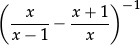
and rewrite it as
= x2 − x.
However one later broadens this use of the equals sign so that “=” simply links two expressions that are “algebraically equivalent”—that is, where one side can be transformed into the other side via the rules of algebra. Any such equation that links two expressions that are algebraically equivalent is called an identity.
2.5.[Subject content: Algebra p. 6]
–model situations or procedures by translating them into algebraic expressions or formulae
This requirement summarises what an idealist would like all pupils to be able to do eventually. However, at present very few pupils ever reach this level of fluency—even at Key Stage 4 (let alone at Key Stage 3: see examples 2.5B and 2.5C below). Hence the requirement needs to be interpreted with care.
One reason for our current limited success is that we fail to separate two stages which have here been combined in the same requirement:
•first learn to translate a numerical procedure, or a sequence of operations, into algebraic form as an expression;
•then learn to equate the results of two such procedures, or to take on board an additional constraint, to derive an equation (or a “formula”).
That is, we pay too little attention to the more modest prerequisite requirement of getting pupils
–to interpret descriptions, or situations, given orally in words and to write down the answers as expressions.
The extent to which we need to rethink current practice is partly illustrated by the following five Year 9 tasks from TIMSS 2011. The first four tasks (2.5A–2.5D) are basic exercises. These are not sophisticated modelling tasks; but they indicate the kind of exercises that we may need to take more seriously, and engage with more systematically, if we are eventually to address the full-blooded requirement at the start of Section 2.5. The fifth example requires one to set up a very simple linear equation and to interpret its solution—and although the comparison countries show that this task is more demanding, the English performance on this problem is in some ways even more telling.
2.5A There were m boys and n girls in a parade. Each person carried 2 balloons. Which of these expressions represents the total number of balloons carried in the parade?
A 2(m + n)B 2 + (m + n)C 2m + nD m + 2n
2.5B A taxi company has a basic charge of 25 zeds and a charge of 0.2 zeds for each kilometre the taxi is driven. Which of these represents the cost in zeds to hire a taxi for a trip of n kilometres?
A 25 + 0.2nB 25 × 0.2nC 0.2 × (25 + n)D 0.2 × 25 + n
2.5C What is the area of the rectangle shown? [A rectangle with length x + 2 and width x is shown.]
A x2 + 2B x2 + 2xC 2x + 2D 4x + 4
2.5D What is the sum of three consecutive whole numbers with 2n as the middle number?
A 6n + 3B 6nC 6n − 1D 6n − 3
2.5E A piece of wood was 40cm long. It was cut into 3 pieces. The lengths in cm are: 2x − 5, x + 7, x + 6. What is the length of the longest piece?
The success rates among Year 9 pupils in our four comparison countries were as follows:
2.5A Russia 90%,USA 88%,Hungary 80%,England 74%,Australia 73%
2.5B Russia 70%,USA 61%,Hungary 50%,Australia 47%,England 45%
2.5C Russia 72%,USA 37%,England 35%,Hungary 30%,Australia 26%
2.5D Hungary 56%,Russia 53%,England 46%,Australia 45%,USA 37%
2.5E Hungary 23%,Russia 22%,Australia 7%,USA 7%,England 3%
Some observers might be satisfied with a 74% success rate for 2.5A. But the Russian, USA, and Hungarian scores should challenge such complacency. (This is a multiple choice question, and the 26% who chose options B, C, or D suggest that a significant number of pupils were simply guessing—so some of the 74% correct will have chosen option A by accident.)
The responses to 2.5B reinforce the impression that most Year 9 pupils in England are very rarely expected to formulate such simple expressions algebraically from a situation given in words. (Note that if 30% of pupils were fairly sure of option A, and the other 70% of pupils were reduced to guessing, then an additional 17.5% of the cohort would select option A by accident—so more than 45% would then have chosen the “correct” option.)
Example 2.5C would seem to be even simpler—provided that pupils can read the simplest diagram and know that “area = length × breadth”.
Setting up an “equation”, or a “formula”, is like writing a sentence. So pupils first need to learn how to “read”, then how to “spell” the ingredient words and how to build up expressions (in a way that respects the conventions of elementary algebra—see Section 2.3). They then need to learn the basic art of naming a variable, and applying a sequence of arithmetical or algebraic transformations to it in a reliable way. We infer that this is either not done, or done in a way that does not allow these key skills to take root.
We have largely resisted the temptation to offer “solutions”. However, as a contribution to the challenge for schools to develop the necessary extended sequence of stages that leads to algebraic fluency, we draw attention to three ingredients that seem to be relatively neglected. These stages relate the need to learn how to “match verbal descriptions with algebraic expressions” (see TIMMS example 2.3A above).
On the simplest level pupils need exercises of the following kind (see example 2.3A above to see why).
Match up each expression on the left with the corresponding English description on the right.
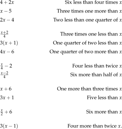
Pupils then need to take the step from “matching up” verbal descriptions and given expressions to reading, or listening to verbal descriptions and reliably translating these into written expressions for themselves. So they need variations on the following activity to cultivate the art of listening, thinking, and interpreting. (We give two contexts for purposes of illustration—but many others can be imagined.) These are intended to be oral challenges, read slowly and clearly, leaving sufficient pauses between successive tasks—with pupils expected to listen and write down “answers” (preferably without the instructions being repeated).
“I’m thinking of a number, which I multiply by 3. Write an expression for my final number.” |
“I’m thinking of a number, which I multiply by 3, and then add 2. Write an expression for my final number.”
“I’m thinking of a number, to which I add 2 and then multiply the result by 3. Write an expression for my final number.”
“I’m thinking of a number, to which I add 2, then multiply the result by 3, and then square the answer. Write an expression for my final number.”
“I’m thinking of a number, to which I add 2, square the result, and subtract 4 times one more than the number I first thought of. Write a fully simplified expression for my final number.”
“A square has sides of length a. Write an expression for its perimeter. Write another expression for its area.” |
“A rectangle has sides of length a and b. Write an expression for its perimeter. Write another expression for its area.”
“A rectangle has sides whose lengths differ by 1. Write an expression for its perimeter. Write another expression for its area.”
“A rectangle has one side twice as long as the other. Write an expression for its perimeter. Write another expression for its area.”
“A rectangle has sides in the ratio 3 : 2. Write an expression for its perimeter. Write another expression for its area.”
Once pupils understand how expressions are constructed they may be in a better position to use this skill to translate a problem, or a result, given in words into an equation or formula, as with such variations on the above oral tasks as the following.
“I’m thinking of a number, which I multiply by 3, and the result is 27. Express this as an equation.” |
“I’m thinking of a number, which I multiply by 3, and then add 2. The result is 41. Express this as an equation.”
“I’m thinking of a number, to which I add 2 and then multiply the result by 3. The result is 39. Express this as an equation.”
“I’m thinking of a number, to which I add 2, then multiply the result by 3, and then square the answer. The result is 36. Express this as an equation.”
“I’m thinking of a number, to which I add 2, square the result, and subtract 4 times one more than the number I first thought of. The result is 144. Express this as an equation.”
“A square has sides of length a. It perimeter is 108. Express this as an equation.” |
“A square has sides of length 2a. Its area is 144. Express this as an equation.”
“A rectangle has sides of length a and b. Its perimeter is 108. Express this as an equation.”
“A rectangle has sides of length a and b. Its perimeter is 10 and its area is 6. Express these facts as two equations in a and b.”
“A rectangle has sides whose lengths differ by 1. Its perimeter is 62. Express this as an equation.”
“A rectangle has sides whose lengths differ by 1. Its area is 56. Express this as an equation.”
“A rectangle has one side twice as long as the other. Its area is 50. Express this as an equation.”
“A rectangle has sides in the ratio 3 : 2. It perimeter is 130. Express this as an equation.”
In the above examples, the numbers have been chosen so that the solutions may be accessed without requiring any special technique. This should allow pupils to check whether the evident numerical solution is consistent with their algebraic formulation. But pupils later need to progress to exercises where the solutions cannot be so easily discerned. The successful solution of any resulting equations will then depend on preparatory algebraic and arithmetical work done elsewhere (especially work with transforming algebraic expressions and with fractions).
In the official Key Stage 3 programme of study, the full version of the requirement given at the start of Section 2.5 is even more ambitious, in that it states that pupils should be taught to:
•“model situations or procedures by translating them into algebraic expressions or formulae and by using graphs.” [emphasis added]
We have already suggested that increased success may depend on separating the art of “formulating a procedure as an algebraic expression” from, and treating it earlier than, “formulating equations”. So the immediate juxtaposition of the two separate stages “expressions and formulae” could be misleading. The final four words above (in bold) would seem to constitute an even more unfortunate juxtaposition, in that two entirely separate requirements that cannot be handled simultaneously have been compressed into a single statement.
The reference to “graphs” suggests that the situation being analysed involves at least two variables. This in turn suggests that this requirement only becomes relevant much later. Long before one can think about “using a graph”, one needs to be able to formulate the relevant algebraic equation in two variables entirely reliably—and this seems likely to take more time and effort than we have realised (see 2.5A–2.5C). Hence schools must be prepared to use their judgement as to when such apparently juxtaposed requirements in the official programme of study have to be separated in time, with the missing stages, or “stepping-stones”, provided internally.
In this instance, the connection with graphs is likely to feature much later. Once pupils have learned to work with linear graphs, one could revisit
•“I’m thinking of a number, which I multiply by 3, and the result is 27.”
and relate the algebraic solution:
Let the unknown number be x.
∴ 3x = 27.
to the point of intersection (9, 27) of the line y = 3x and the ordinate y = 27.
Later in Key Stage 3, or in early Key Stage 4 (see the third, fourth and fifth requirements in section 2.7 below), pupils might relate the problem
“I’m thinking of a number, to which I add 2, then multiply the result by 3, and then square the answer. The result is 36. Express this as an equation.”
to the intersection point (2, 36) of the graph of y = 9(x + 2)2 and the ordinate y = 36.
In the same spirit, the problem:
“A rectangle has sides whose lengths differ by 1. Its area is 56. Express this as an equation.”
could be linked to the positive intersection point (7, 0) (after rejecting (−8, 0)) of the graph of y = x2 + x − 56 with the x-axis y = 0.
And having learned to solve quadratic equations at Key Stage 4, pupils might relate
“A rectangle has sides of length a and b. Its perimeter is 10 and its area is 6. Express these facts as two equations in a and b.”
to the equation x2 − 5x + 6 = 0 (whose roots are a and b). Some pupils could then explore the general question of whether knowing the sum a + b and the product ab of two unknowns is always sufficient to determine a and b.
Teachers should know that this latter idea (namely that a rectangle is determined by its area and its semi-perimeter) is more important than one might think—both historically and at higher levels. The ancient Babylonians and Greeks both tackled quadratics in this way (among others).
Babylonian: around 1700 BC The Babylonian approach was eclectic, and essentially algebraic, but without symbols. The problems were expressed in words, and the solution methods were given as recipes applied to the particular numbers in the problem; but the recipes were so formulated that they would still work if the particular numbers were changed. They addressed a remarkable variety of problems which correspond to what we would call “quadratic equations”. Otto Neugebauer, the leading historian of such matters in the first half of the 20th century, catalogued hundreds of examples in what he called “normal form”, where two numbers were to be found if their product and their sum (or difference) were known. Neugebauer also found countless exercises designed to train young scribes how to reduce other sorts of quadratic problems to this “normal form”.
Greek: around 300 BC The Greek approach is harder to explain briefly, because it was expressed purely geometrically (for they had no way of writing algebraically). If we cheat a little and describe the steps in their method partly algebraically, their “normal form” for a quadratic problem was to imagine a line segment broken in to unequal lengths (so of length a + b, with a > b):
•to construct the midpoint and then construct the square on half of the complete segment
•to construct the “a by b” rectangle with the two unequal segments as sides
•to subtract the rectangle from the square
•to construct the square which was equal to this difference (whose side was therefore “(a − b)”)
•to combine the segments of length (a + b) and of length (a − b) to find a; then find b.
All of this was done strictly geometrically—though we would write the process algebraically as
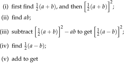
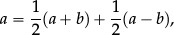
and subtract to get
When pupils proceed beyond GCSE, they will need to know that:
•If a quadratic x2 + dx + e has roots a and b, it can be factorised as
x2 + dx + e = (x − a)(x − b);
and multiplying out the RHS shows that
d = −(a + b)ande = ab.
Hence once we know the quadratic, we already know the sum and product of the roots, and “solving the equation” is a way of going from knowing “the sum and product of the roots” to finding the roots themselves.
•Though the Babylonians and Greeks did not know it, they had hit upon something important. For if a cubic x3 + dx2 + ex + f has roots a, b and c, then it can be factorised as
x3 + dx2 + ex + f = (x − a)(x − b)(x − c);
and multiplying out the RHS shows that
d = −(a + b + c),e = ab + bc + ca, and f = −abc.
Hence once we know the cubic, we already know the sum of the roots (−d), the product of the roots (−f), and the sum of the products in pairs (e). So “solving a cubic equation” requires us to find a way of going from knowing “the sum of all three roots, the product of all three roots, and the sum of the products in pairs” to finding the three roots themselves.
2.6.[Subject content: Algebra p. 6]
–use algebraic methods to solve linear equations in one variable (including all forms that require rearrangement)
Pupils will no doubt already be familiar with the way general results such as C = 2πr can be expressed using letters; but in such a formula, the letters stand for familiar entities (the radius r of the circle, and its circumference C). In contrast, solving linear equations in one unknown may well be pupils’ first encounter with symbols being used to encode information about completely unknown entities. So this is likely to be the setting in which key ideas about algebra are internalised—and where misconceptions may well take root.
We have seen (Part II, Section 2.2.2.2) that “to solve equations” means to solve exactly—by algebraic methods. We start out with an equation which has an unknown set of solutions, or possible values for the unknown “x”. “Solving the equation algebraically” is a process which pins down the unknown “x” by exploiting two kinds of “moves”.
•The first kind of move allows us to replace any constituent expression on either side of the equation by another expression which is algebraically equivalent to it (for example, we can “collect up” separate multiples of the unknown “x” into a single term). Because this kind of move is reversible, we know that exactly the same values of the unknown “x” satisfy the new equation as satisfied the old equation.
•The second kind of move is to subject both sides of the equation to the same operation (for example, we can add the same quantity to both sides, or multiply both sides by the same quantity). As long as this operation is reversible (as it always is if we add or subtract the same quantity to both sides, or if we multiply or divide both sides by a given expression that is never equal to zero), then we can again be sure that exactly the same values of the unknown “x” satisfy the new equation as satisfied the old equation.
Pupils need to learn not only to transform equations according to these rules of algebra, but also to recognise any pair of equations which are algebraically equivalent. Thus they should be faced with such tasks as:
Match up each equation on the left with the equation(s) on the right to which it is equivalent.
Pupils also need lots of equations to solve, and standard contexts in which they learn to set up and solve equations which reveal things that were not previously clear and that are vaguely interesting. We offer a sequence of problems based on one idea—but there are dozens of other possible settings.
(a)I start with the fraction . I wish to add the same amount to the numerator and to the denominator so that the result is equal to  . What amount should I add?
I then start with the fraction . I wish to add the same amount to the numerator and to the denominator so that the result is equal to . What amount should I add?
I then start with the fraction . I wish to add the same amount to the numerator and to the denominator so that the result is equal to . What amount should I add?
I then start with the fraction . I wish to add the same amount to the numerator and to the denominator so that the result is equal to . What amount should I add?
(b)I start again with the fraction . I want to add some amount a to the numerator and subtract the same amount from the denominator to make the result equal to . Find a.
I then start with the fraction . I want to add some amount b to the numerator and subtract the same amount from the denominator to make the result equal to . Find b.
I then start with the fraction . I want to add some amount c to the numerator and subtract the same amount from the denominator to make the result equal to . Find c.
I then start with the fraction . I want to add some amount d to the numerator and subtract the same amount from the denominator to make the result equal to . Find d.
I then start with the fraction . I want to add some amount e to the numerator and subtract the same amount from the denominator to make the result equal to 1. Find e.
2.7.[Subject content: Algebra pp. 6-7]
–work with coordinates in all four quadrants
–reduce a given linear equation in two variables to the standard form y = mx + c; calculate and interpret gradients and intercepts of graphs of such linear equations numerically, graphically and algebraically
–recognise, sketch and produce graphs of linear and quadratic functions of one variable with appropriate scaling, using equations in x and y in the Cartesian plane
–use linear and quadratic graphs to estimate values of y for given values of x and vice versa and to find approximate solutions of simultaneous linear equations
–model situations or procedures by translating them into algebraic expressions or formulae and by using graphs
–interpret mathematical relationships both algebraically and graphically
–find approximate solutions to contextual problems from given graphs of a variety of functions, including piece-wise linear, exponential and reciprocal graphs
[Ratio, proportion and rates of change p. 7]
–solve problems involving direct and inverse proportion, including graphical and algebraic representations
2.7.1This collection of requirements linked to graphs needs to be treated with extreme care. The first requirement makes perfect sense. The first half of the second requirement is equally standard; but the second half is already far from clear. And as one reads on, the meanings become more opaque and the stated goals appear progressively more optimistic, or overblown at this level. For example, we have already seen that direct proportion is hard, and that its “graphical and algebraic representation” may be more appropriate at Key Stage 4 (for more confident pupils); so the inclusion of this requirement for “inverse proportion” may need to be taken with a pinch of salt.
In short, we would urge schools to sift out what clearly belongs to Key Stage 3 and to teach it well. Where material seems out of place at Key Stage 3, and where the listed material in standard type in the Key Stage 4 programme of study either repeats it verbatim or does not take it much further, work at Key Stage 3 should perhaps be limited to “preparatory” experience that can then be built on in Years 10 and 11.
2.7.2The first requirement could be interpreted as being limited to work with individual points. However, one of the characteristic features of coordinate geometry and equations is that they are ways of working with groups of points or lines.
•An equation represents the set of all points (x, y) that satisfy the equation.
•To find the equation of a straight line we use the known coordinates of two given points and the unknown coordinates of a third variable point (x, y) which lies on the line.
•And we think about the solutions of simultaneous equations as the point, or points, where two or more lines or curves intersect.
So pupils need to learn to work with several points at once. The gulf between understanding ideas or methods in isolation (one-piece jigsaws) and being able to handle two or more simple ideas at once is indicated by the following item for Year 9 pupils in TIMSS 2011.
2.7.2A (0, −1), (1, 3) Which equation is satisfied by both of these pairs of numbers (x, y)?
A x + y = −1B 2x + y = 5C 3x − y = 0D 4x − y = 1
2.7.2A Russia 53%,USA 38%,Hungary 29%,England 24%,Australia 22%
So before pupils begin to work with equations, basic work with coordinates should include learning to think about the “relative position” of groups of points. For example:
•One may give the coordinates of three vertices of a square, and require them to be located, and the coordinates of the fourth (unspecified) vertex to be found and the vertex marked.
•One may specify the coordinates of two neighbouring vertices of a square (for example, (−4, 2) and (−3, −3)), and ask for the possible coordinates of the other two vertices.
•One may specify the coordinates of two opposite vertices of a square and require that the other two vertices be marked and their coordinates found.
That is, pupils need lots of work which not only establishes the underlying conventions, but which teaches them to “see”, and to think about, groups of points (and lines) that are related to each other in some way.
2.7.3After sufficient experience imagining, and locating individual points and groups of points in all four quadrants, pupils will be well-placed to think about what links a given set of points (preferably given as a list, rather than as a table) such as:
(−6, −3), (−4, −2), (−2, −1), (0, 0), (2, 1), (4, 2), (6, 3), (8, 4).
Plotting points should convey the idea that they appear to lie on a line, and that
each time the x-coordinate increases by 2, the y-coordinate increases by 1 (“along 2, up 1”).
One can then ask for the coordinates of intermediate points that lie on the same line, both to establish the possibility of fractional values (such as  , or
, or  , or
, or  ), and to extract
the unit step: “along 1, up ”.
Pupils can go further and then find  (“along , up ”), and
  (“along , up ”), etc.. They should also be challenged to identify points on the same line with much more distant coordinates (such as (100, 50), or (−200, −100)).
Once these ideas (that the line extends indefinitely, and that it includes points that are as close together was we choose) have been firmly established, one can
•look for ways of relating x- and y-coordinates of points which lie on the line,
•obtain the usual equation “y = x”, and
•check that every point on the line satisfies this equation, and that every point whose coordinates satisfy the equation must lie on the line.
It may be necessary to repeatedly reinforce the idea that
•the collection of points on the line, and
•the collection of points whose coordinates (x, y) satisfy the equation y = x
are the same (i.e. that points lie on the line precisely when their coordinates satisfy the equation): that is, that the equation provides an algebraic way of reasoning about, and calculating with, the geometrical line.
This whole sequence can then be repeated for a new set of points
(−6, −2), (−4, −1), (−2, 0), (0, 1), (2, 2), (4, 3), (6, 4), (8, 5).
Again, plotting points will indicate that the points lie on a line, that whenever the x-coordinate increases by 2, the y-coordinate increases by 1 (“along 2, up 1”), and that this line can never meet the first line (since the first line goes through (−6, −3) and follows the rule “along 2, up 1”, whereas the second line follows the same rule “along 2, up 1”, but goes through a point (−6, −2) which does not lie on the first line). Again one can ask pupils to find the coordinates of intermediate points on the line, and for points on the line with much more distant coordinates (such as (100, 51), or (−200, −99)), and can then obtain the usual equation y = x + 1. The significance of the parameters m = , and of c = 1 can be established. And everything can be reinforced by considering the new set of points
(−6, −5), (−4, −4), (−2, −3), (0, −2), (2, −1), (4, 0), (6, 1), (8, 2).
In making sense of the linear equation y = mx + c, pupils need to internalise the significance
•of c (as the y-coordinate of the point where the line crosses the y-axis).
They also need sufficient experience to establish a clear mental image of how the parameter m affects the visual impression of the represented line (assuming that equal scales are used on both axes), so that they distinguish:
•lines in which m = 1 (rising to the right at 45°),
•lines with 0 < m < 1 (rising to the right less steeply than m = 1)
•lines with m > 1 (rising to the right more steeply than m = 1), and
•lines with m < 0 (falling as one moves to the right).
Schools will need to decide for themselves how much of what follows is best handled at Key Stage 3 and how much fits more naturally within Key Stage 4. But at some point, once the basic ideas have been grasped, pupils need to do lots of work in the opposite direction:
•starting with linear equations given in a variety of forms (including with terms in “x” and in “y” on both sides of the equation, and where the y-terms may have any positive or negative coefficient),
•reducing the given equation to the “standard form y = mx + c” (or “x = a”)
•and then sketching the line.
Pupils eventually need to be able to find the equation of a line which satisfies certain conditions, such as:
(a)passing through a given point with a given gradient m,
(b)with a given y-intercept (0, c) and passing through a given point,
(c)with a given gradient m and a given x-intercept (a, 0),
(d)with a given x-intercept and passing through a given point,
(e)passing through two given points.
2.7.4Once the basic language of straight line graphs and linear equations has been established, pupils are ready to explore the wealth of problems whose natural representation is in terms of linear equations and straight line graphs.
We have already seen how this arises whenever two quantities are related in such a way as to be “in proportion”, so that doubling the first quantity (such as the number of hours worked) leads to a doubling of the second quantity (the pay that is earned: see Section 1.9.2 above and Part II, Section 2.2.1). This is clearly relevant to the last requirement listed at the start of Section 2.7. If two different quantities vary “in proportion”, and we know two corresponding numerical values—one of the first kind (a), and one of the second kind (c),
a ![]() c
c
then any two corresponding unknown amounts x and y (one of the first kind and the other of the second kind) provide the third and fourth vertices of our “rectangular template”
x ![]() y
y
and the proportion
x : a = y : c
translates into an equality of ratios, or fractions

which in turn gives rise to the linear equation

with “constant of proportionality”, or gradient, .
Such examples also arise whenever one changes units. If the units belong to the same system, then the constant of proportionality will be exact, and relatively simple. For example, when changing from centimetres to metres, M metres becomes C = 100M centimetres. But if the units come from different systems, then we usually simplify by using a convenient approximation to the “constant of proportionality”. For example, when changing from miles into kilometres, M miles is generally taken to be K =  Mkm, where we use 1.6 as the approximate scale factor in place of the messy actual value of “1.609344 to 6 decimal places”.
However, just as most straight line graphs y = mx + c do not have c = 0, so we must expect most linear relations to occur with a built-in “offset” c ≠ 0. This offset can be interpreted as saying that the two scales we are comparing need to be “re-aligned”. For example, the equation which relates the temperature F in Fahrenheit with the temperature C in Centigrade, or Celsius, is

Here the “+ 32” arises because there is no obvious “zero” for measuring temperature; the Celsius scale uses the freezing point of water as 0°C, whereas the Fahrenheit scale locates this at 32°F. (In this instance, although the units arise from different systems, the scale factor “ ” is exact, because the Celsius scale from 0°C to 100°C matches up uniformly with the Fahrenheit scale from 32°F to 212°F, so that each 1°C corresponds to exactly 1.8°F.)
A straight line graph tells us that there is a “linear relation” between x and y even if the line does not go through the origin. Most instances where there is some hidden proportion occur with an “offset” (that is, with c ≠ 0). A good example is the graph which underlies example 2.5B:
2.5B A taxi company has a basic charge of 25 zeds and a charge of 0.2 zeds for each kilometre the taxi is driven. Which of these represents the cost in zeds to hire a taxi for a trip of n kilometres?
A 25 + 0.2nB 25 × 0.2nC 0.2 × (25 + n)D 0.2 × 25 + n
Here the cost of a journey is directly proportional to the distance travelled—except for the addition of a “basic charge of 25 zeds”; hence the charge “y zeds” for a journey of length x km (priced in “zeds”—the universal currency in TIMSS problems) is given by
y = 0.2x + 25
which is better written without decimals as
Mathematics teachers need to remember that scientists, engineers and others will go to almost any lengths to reduce more complicated relationships to ones that give rise to straight line graphs—because empirical laws are easiest to discern, or to confirm, if the approximate data can be plotted to look as though it fits on a straight line. For example, if a scientist believes the data should satisfy an equation of the form y = kx2 for some positive constant value k, then rather than plotting x against y and having to identify a parabola, they might well
•plot values of x2 against values of y and hope to see a straight line with gradient k, or
•plot log(x) against log(y) and expect to see a straight line with gradient 2 and with y-intercept c = log(k).
2.7.5Such connections and applications should be part of any treatment of linear equations at Key Stage 3 and Key Stage 4, and this presumably covers at least part of what is meant by the fifth requirement listed at the start of Section 2.7 (“model situations …”), and also the sixth requirement (“interpret mathematical relationships … ”).
2.7.6The third and fourth requirements at the start of Section 2.7 mention quadratic functions and quadratic graphs. These references need to be interpreted with care.
The new GCSE specification (and hence the programmes of study for Key Stage 3 and 4) deliberately downplay premature reference to abstract “functions”, and to function notation—such as f(x). Instead, the programmes of study would appear to be designed to emphasise the use of such ideas in concrete form before abstractions such as f(x) are introduced in Year 12 (though there is nothing to prevent a school from doing both prior to GCSE).
So when the word “function” appears in the context of linear and quadratic functions, it is being used informally, indicating that the curriculum should prepare the ground for a more abstract formulation in Year 12. In particular, work at Key Stage 3 should take account of the fact that GCSE will no longer expect pupils to use the abstract notation f(x). Nor will pupils be expected to make sense of general transformations of coordinates
•moving the y-axis by rewriting the given expression for the function in the form f(x ± a), or
•moving the x-axis by rewriting the given expression for the function in the form f(x) ± a, or
•moving both axes at once by rewriting the given expression for the function in the form f(x ± a) ± b.
Instead, by the end of Key Stage 4, pupils who expect to take Higher tier GCSE need to be able to implement such transformations in the contexts of specific linear, or quadratic, or trig functions. Pupils will therefore work with particular functions f and with particular numerical values of the parameters a and b. But for convenience we summarise these specific numerical examples by giving them in general symbolic form.
•The general linear equation y = mx + c can be seen to be essentially the same as Y = mX in two obvious ways:
–by moving the origin to (0, c), and setting Y = y − c, and X = x, and also
–by moving the origin to  , and setting Y = y, and X = x +
  .
.
•Pupils need exercises that lead them to recognise that any given quadratic equation behaves essentially just like y = x2 or y = −x2.
–The first step is to understand the prototype of all quadratics, namely y = x2,
*to appreciate its symmetry about the y-axis (giving the same y value for ± x)
*to recognise how it “sits on” (or is tangent to) the x-axis
*how this relates to the fact that squaring values of x between −1 and 1 produces a smaller output x2, while squaring values of x which are greater than 1 or less than −1 gives rise to larger and larger outputs x2.
–This analysis can then be extended to graphs whose equation has the form y = x2 + c, where c may be either positive or negative, and where moving the origin to (0, c) corresponds to a change of coordinates: Y = y − c, X = x, so that the original equation y = x2 + c becomes Y = X2.
–The same idea extends to equations of the form y = (x − a)2, and to those of the form y = (x − a)2 + c.
–And one can show (via particular numerical examples) how any given quadratic equation y = x2 + bx + c can be rewritten in such a form by “completing the square”
so that the original equation becomes Y = X2, where

and
–Later (perhaps in Year 12) those who enjoy algebra can discover how the general quadratic y = ax2 + bx + c can be rewritten as
which turns into Y = X2 after shifting the origin and dividing both x and y by “a”. Hence, although some quadratics appear tall and skinny, while others appear short and fat, all parabolas are in fact similar, just as all circles, or all squares are similar.
2.7.7The requirement to work with “given graphs of a variety of functions, including piece-wise linear, exponential and reciprocal graphs” needs to be interpreted carefully, in the spirit of 2.7.6. Given the apparent ruling about “functions” in general at GCSE, this stated requirement would seem to have limited relevance at Key Stage 3. Even at Key Stage 4 it may mean little more than that pupils
•should ideally be familiar with the graph of y =  and its obvious variants (such as y =
  , or possibly y =
  );
);
•should have some experience of such graphs as y = (1.05)x, that arise when exploring how an investment, or a debt of £1 would grow in x years at 5% per annum; and
•should be prepared to make sense of natural problems where the given data happen to give rise in some way to a graph that is (for example) piece-wise linear.
2.7.8The fourth requirement listed at the start of Section 2.7 states that
•“pupils should be taught to use linear and quadratic graphs to estimate values of y for given values of x and vice versa, and to find approximate solutions of simultaneous linear equations.”
The seventh listed requirement at the start of Section 2.7 also mentions finding “approximate solutions”.
These two requirements appear to confuse two quite different things—each of which is valuable, but whose combination here is potentially confusing.
It is important for pupils to learn to “read a graph”. By this we mean:
•that pupils be confronted with a graph whose equation is unknown,
•that they be given a value a of x, and have to trace the corresponding abscissa x = a to see where it hits the graph, and then to trace the corresponding ordinate from that point to the y-axis to estimate the value of y corresponding to x = a (using their eyes, or their fingers, or a carefully positioned—preferably transparent—ruler), and
•that they be given a value b of y, and have to trace the corresponding ordinate y = b to find all the points where it hits the graph, and then to trace the corresponding abscissas from these points on the graph to the x-axis to estimate all the values of x corresponding to y = b.
An entirely separate (and equally important) requirement is, given a formula or equation relating x and y, to substitute values for x, so that expressions involving x become numerical expressions, and so to use arithmetic to discover what this says about the corresponding value of y (see Section 2.4.2 above). Note however, that in this process the calculations are exact, not estimates.
The listed requirement appears to confound these two very different, and entirely admirable, activities, by suggesting that pupils should engage in such “estimation” with “linear and quadratic graphs”. But if we know that we are working with a “linear graph” or a “quadratic graph”, then we must know its equation—so substitution becomes an exact calculation, rather than a matter of estimation—with one exception.
•If the equation is linear, then given a value of x, pupils should calculate an exact value of y; and given a value of y, one can equally demand that they calculate an exact value of x.
•If the equation is quadratic, then given a value of x, pupils should calculate an exact value of y.
•Hence, the only obvious scope for “estimating values” would seem to arise in asking, for a given quadratic graph or equation,
–“Which possible values of x give rise to a given value of y?”
This is an excellent requirement (namely to draw the relevant ordinate parallel to the x-axis, to estimate where it cuts the graph, and to infer the approximate values (if any) of x—which one can then check by substituting the estimated values in the known equation).
The final part of the fourth requirement
“to find approximate solutions of simultaneous linear equations”
might be fine if it was stated at a point where pupils could see how it links up with
finding the exact solution (by eliminating a variable).
But there is no mention of this requirement at Key Stage 3, so the requirement to address the significant challenge of working with simultaneous equations purely in order to find approximate solutions seems seriously premature.
At Key Stage 4, Higher tier candidates are expected to find the intersection points of a line and a circle, so it makes sense to consider how to prepare the ground for such pupils at Key Stage 3. In general one would eventually like all pupils to understand that
•the solutions of simultaneous equations
correspond to
•the coordinates of points where two lines or curves meet.
This is an important idea, provided it is not misrepresented as an alternative to “solving the equations algebraically”. So at the point where simultaneous linear equations are to be solved exactly, pupils need to understand
•that the two linear equations correspond to two straight lines in the plane,
and
•that the output from the solving process is precisely the coordinates of the point where the two lines cross.
So as and when a class is ready to handle “elimination of a variable” in order to find the exact solution, it makes sense for them
•to draw the two lines,
•to recognise that the solution (x, y) that they seek corresponds to the coordinates of the point where the two lines cross, and
•to estimate the solution that is being sought (as a guide for what they should expect to emerge from the subsequent algebraic exact calculation).
They would then be in a good position to confront the algebraic challenge of “how to eliminate a variable”, and to use this new-found skill to tackle lots of lovely problems. But there is something wrong with a programme that requires pupils to find “approximate” solutions while not revealing the fact that one can find the exact solution.
One would also like pupils to tackle problems where this geometrical interpretation is an essential part of the problem (for example, where they are given the coordinates of three vertices of a triangle, and are required to find the coordinates of the point where two medians meet). However, such problems are rather hard precisely because they require pupils to coordinate several steps (find the coordinates of the midpoints of the sides; find the equations of the two medians; solve these two simultaneous equations; extract the coordinates of the point where they cross).
2.8.[Subject content: Algebra p. 7]
–generate terms of a sequence from either a term-to-term rule or a position-to-term rule
–recognise arithmetic sequences and find the nth term
–recognise geometric sequences and appreciate other sequences that arise.
Work with sequences provides valuable opportunities:
•to revise and to strengthen arithmetic
•to cultivate the ability to notice basic patterns (constant, linear, powers, exponentials)
•to discover how geometrical and combinatorial sequences often give rise to familiar integer sequences
•to express numerical patterns algebraically
•to link discrete sequences with work on functions and graphs.
For example,
•if a formula is given for the nth term, then finding the succession of terms is an exercise in substituting easy numerical (integer) values into an expression;
•if the first few terms of a sequence are given (whether 2, 4, 6, 8, … , or 4, 7, 10, 13, … , or 0, 3, 8, 15, … , or 1, 3, 7, 15, … , or 2, 5, 13, 35, …), then it is an excellent exercise to think of the simplest algebraic expression that could generate the given sequence.
A sequence
x1, x2, x3, x4, x5, …
is a way of presenting an endless amount of information in a single list. There are two quite different ways of specifying the terms of such a sequence.
The first, and most primitive, way is to give the first few terms and then to specify a term-to-term rule (or “recurrence relation”) that tells you how to work out the next term from the ones you already know. For example,
•x1 = 3, xn+1 = 2xn defines the sequence 3, 6, 12, 24, 48, … ;
•x1 = x2 = 1, xn+1 = xn + xn − 1 defines the sequence 1, 1, 2, 3, 5, 8, 13, …
•x1 = 2, xn+1 = 3xn − 2n defines the sequence 2, 4, 8, 16, 32, … .
This first approach allows you to continue the sequence as far as you like, and determines the 10th, the 100th, and the 1000th terms uniquely. However, in order to find the 1000th term we first have to calculate the 1st, the 2nd, the 3rd, … , and the 999th terms. In other words, we can generate terms of the sequence, but it may not be easy to obtain a proven closed formula giving the nth term of the sequence as a formula in terms of n. We may think we can guess how the sequence is behaving, but we are unlikely to be able to prove anything about the sequence as a whole.
•In the first of our three examples above, we can see that:
the first term x1 = 3 is doubled n − 1 times to get the nth term, so xn = 3 × 2n − 1.
•In the second example, it is easy to generate more and more terms, but it is quite unclear how to write the nth term as a closed formula in terms of n.
•In the third example, it is easy to guess that the closed formula for the nth term looks as though it “has to be” xn = 2n, but it is not at all clear how to prove that this is correct.
In short, a term-to-term rule is easy to use, but it is inefficient; and it gives us no way of reasoning in general about the nth term.
The second (and generally more powerful) way to specify a sequence is by a position-to-term rule, which tells you how the nth term can be calculated directly in terms of n. That is, the sequence of terms
x1, x2, x3, x4, x5, … , xn, …
is simply a listing of the outputs for a single rule, or function f, by listing
f(1), f(2), f(3), f(4), f(5), … , f(n), … .
A position-to-term rule may be given explicitly by a formula—as with
•the sequence of squares, where xn = n2, or
•the sequence of powers of 2, where xn = 2n.
But a position-to-term rule may also define a sequence intrinsically, with the nth term being defined to be a number which can be calculated from some algebraic procedure, or from some geometrical configuration. For example:
•Let the nth term tn of a sequence be defined to be equal to the sum of the first n positive integers. Then
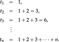
•Let the nth term cn of a sequence be defined to be the number of chords that can be created by joining pairs of points chosen from n points marked on a circle. Then
1 point on a circle gives rise to c1 = 0 chords;
2 points on a circle give rise to exactly c2 = 1 chord;
3 points on a circle give rise to c3 = 3 chords; etc..
•Let the nth term fn of a sequence be defined to be equal to the number of positive factors of n. Then
f1 = 1, f2 = 2 (factors 1 and 2); f3 = 2 (factors 1 and 3), f4 = 3 (factors 1, 2, and 4); … .
In these three examples, the position-to-term rule tells us exactly how to find each term; but the underlying function, or rule, is given as a process or a recipe, rather than as a formula. This makes it possible to generate
•the first sequence, whose nth term is sum of the first n positive integers, by simply working out any term we need:
1, 1+2 = 3, 1+2+3 = 6, 1+2+3+4 = 10, 1+2+3+4+5 = 15, 1+2+3+4+5+6 = 21, … .
•the second example, whose nth term is equal to the number of chords created by n points on a circle:
0, 1, 3, 6, 10, 15, …
•the third sequence, whose nth term is equal to the number of positive factors of n:
1, 2, 2, 3, 2, 4, 2, 4, 3, 4, 2, … .
Each sequence is well-defined, but we are not given either a term-to-term rule or a closed formula for any of the sequences. So any claims we might wish to make about how each sequence behaves must be deduced from the given algebraic or geometrical definition.
An arithmetic sequence
c, c + m, c + 2m, c + 3m, c + 4m, …
is one that goes up in constant steps: that is, where the term-to-term rule for the sequence is simply
“add m” for some fixed constant m.
The nth term is determined by the first term c and the n − 1 steps of size m that take us from the 1st term to the nth term:
∴ the nth term is equal to “c + (n − 1)m”.
The prototype of every arithmetic sequence is the familiar counting sequence
0, 1, 2, 3, 4, 5, 6, 7, 8, 9, 10, … .
The general arithmetic sequence arises from the counting sequence
•by first multiplying the whole sequence by m (to get
“0, m, 2m, 3m, 4m, … , (n − 1)m, …”)
•then adding c to every term (to get
“c, c + m, c + 2m, c + 3m, c + 4m, … , c + (n– –1)m, …”)
If we think of the nth term “c + (n − 1)m” as a function of x = n − 1, then we see that the sequence lists the values of “y = mx + c” for integer values of x. So the sequence corresponds to the sequence of points for x = 0, x = 1, x = 2, etc. on the straight line y = mx + c; hence another name for an “arithmetic sequence” is a “linear sequence”.
In general, once we have a closed formula for the nth term of a sequence, we can treat n = x as the dependent variable and “plot the graph of the sequence” as a “point graph”, with one graph point for each positive integer value of x = n. The “common difference” m is then the “gradient” of this point graph (for every unit step to the right in the positive n = x direction, the point graph jumps up distance m in the y direction), and the initial value c is the point at which the point graph hits the y-axis. The tradition of using “a” for the first term in place of “c”, and using “d” for the common difference in place of “m” makes it much less likely that pupils will appreciate this important connection.
c, cr, cr2, cr3, cr4, cr5, …
is one for which the term-to-term rule for the sequence is simply
“multiply by r” for some fixed constant r.
Hence the nth term is completely determined:
•by the first term c, and
•by the n − 1 steps “multiply by r” that take us from the 1st term c to the nth term.
•∴ the nth term is equal to “crn − 1”.
If we think of the nth term “crn − 1” as a function of x = n − 1, then we see that the sequence is specified by the two constants c and r, and lists the values of y = c · rx for integer values of x (starting at x = 0). Because the term number “n” appears as an exponent, a geometric sequence is also called an exponential sequence.
In the third requirement listed at the start of Section 2.9 it is unclear what exactly is meant by
“and appreciate other sequences that arise”.
However, these “other sequences” should certainly include:
•linear sequences (or arithmetic sequences)
•quadratic sequences, like the sequence of squares:
12, 22, 32, 42, 52, … n2, …
•the sequence of triangular numbers
0, 1, 3, 6, 10, 15, 21, …
•the sequence of cubes:
1, 8, 27, 64, 125, 216, 343, …
1, 1, 2, 3, 5, 8, 13, 21, 34, … .
School mathematics often gives the impression that all sequences are polynomial sequences—that is, sequences where the nth term is a polynomial function of n, as with
•linear sequences (or arithmetic sequences)
•quadratic sequences, like the sequence of squares
12, 22, 32, …, n2, …
or the sequence of triangular numbers
1, 1 + 2, 1 + 2 + 3, … , 1 + 2 + 3 + … + n =  , …
, …
•the sequence of cubes
13, 23, 33, … , n3, ….
However, nature (and mathematics) often prefers geometric or exponential sequences, such as
the powers of 2:
2, 4, 8, 16, 32, 64, 128, … ,
or the Fibonacci sequence:
1, 1, 2, 3, 5, 8, 13, 21, 34, … .
One key distinction between the two types of sequences becomes apparent if we compare what happens when we look at the sequence of “term-to-term differences” for each type of sequence.
(a) The sequence of “term-to-term differences” for a linear sequence, such as
2, 4, 6, 8, 10, 12, … ,
gives rise to a constant sequence of differences
2, 2, 2, 2, 2, … .
The sequence of “term-to-term differences” for a quadratic sequence, such as
1, 4, 9, 16, 25, 36, …
gives rise to a linear sequence of differences
3, 5, 7, 9, 11, … ,
whose own sequence of differences (or “second differences”) is then constant
2, 2, 2, 2, … .
The sequence of “term-to-term differences” for the quadratic sequence of triangular numbers
0, 1, 3, 6, 10, 15, 21, …
gives rise to a linear sequence of differences
1, 2, 3, 4, 5, 6, … ,
whose own sequence of differences is then constant
1, 1, 1, 1, 1, … .
(b) The sequence of “term-to-term differences” for a geometric sequence behaves quite differently. If we consider the geometric sequence of powers of 2:
2, 4, 8, 16, 32, 64, 128, …
then the sequence of “term-to-term differences” gives rise to
2, 4, 8, 16, 32, 64. …
which is the same as the original sequence, so taking second and third differences will never lead to anything simpler.
If we consider the Fibonacci sequence:
1, 1, 2, 3, 5, 8, 13, 21, 34, …
Then taking differences gives rise to
0, 1, 1, 2, 3, 5, 8, 13, …
which is essentially the same sequence again. Hence taking second and third differences will never lead to anything simpler.
In short, taking differences repeatedly for a polynomial sequence seems to lead eventually to a constant sequence, whereas the sequence of differences for a geometric (or exponential) sequence leads only to something closely related to the original sequence (from which it never escapes).
12http://timss.bc.edu/timss2011/international-released-items.html
13http://timss.bc.edu/timss2011/international-released-items.html
14http://www.manchestereveningnews.co.uk/news/greater-manchester-news/cool-cash-card-confusion-1009701
15https://www.gov.uk/government/uploads/system/uploads/attachment_data/file/335158/PRIMARY_national_curriculum_-_Mathematics_220714.pdf
16http://www.jmc.org.uk/documents/JMC_Report_Digital_Technologies_2011.pdf
17http://education.lms.ac.uk/wp-content/uploads/2012/02/Gardiner_on_JMC.pdf
18http://www.cambridgeassessment.org.uk/news/playlist/view/maths-podcasts/
19http://www.eamesoffice.com/the-work/powers-of-ten/
20http://timss.bc.edu/timss2011/international-released-items.html

