


Geometry should be one of the highlights of mathematics teaching in lower secondary school.
•The subject matter is intuitively appealing and practical.
•It offers extensive scope for drawing intriguing figures, for implementing unexpected constructions, and for making pleasing—even beautiful—models.
•The tools and principles which allow us to analyse this wonderful world exactly are surprisingly simple and accessible.
•All pupils can calculate some surprising things, can solve some interesting problems, and can prove some strikingly useful results; and more confident pupils can prove a wide range of remarkable and unexpected facts.
•Applications to the world around us are immediate, convincing, and impressive.
•The material of school geometry captures the spirit of mathematics better than almost any other part of elementary mathematics.
One would be hard-pressed to discern these strengths in the published programme of study. In particular, there is little emphasis on drawing and making, no clear indication of the intended deductive structure for geometry, and there is no mention of applications to the world around us. But the Good News is that the official programme is compatible with an approach based on the above bullet points—provided schools do not simply mimic the printed sequence of official requirements.
There is considerable confusion over geometry in many apparently authoritative pronouncements—including the requirements listed in the official Key Stage 3 programme of study. To understand why, teachers need to know how we got where we are. So we begin with a thumbnail sketch of some of the relevant historical and pedagogical roots of the current approach to school geometry in England.
School work with number and algebra tends to be relatively “one dimensional”. Typical problems look fairly familiar, and can usually be solved by implementing some well-rehearsed “linear” procedure.
•One is told what is to be calculated (the goal).
•It is usually fairly clear where to begin.
•And with sufficient practice, one can more-or-less follow one’s nose to get from the start to what is required.
Real mathematics is not like this, and is more like what secondary school geometry ought to be.
•We are given some information about a two- or three-dimensional configuration or shape.
•We are asked to calculate something, or to prove some fact.
•We have to draw and edit a diagram as a guide.
•Then we are left to find for ourselves
(i)a suitable feature of the figure that might serve as a starting point, and
(ii)a sequence of steps from this (elusive) start to what is required.
•Because figures and diagrams are in two dimensions, there is often no clear starting point, and no obvious route from start to finish.
For pupils (and teachers) who have come to see school mathematics as a collection of predictable, one-dimensional procedures, this experience is unsettling. The given figure may appear elementary; and one may understand what is wanted. But one often has no idea where to begin, or how to proceed. As we noted in Section 2.3 of Part II (Solving problems), in such a setting it does not take much for a routine exercise to become a frustratingly elusive problem. Geometry reveals this distinction more strongly than most other parts of elementary mathematics.
Most mathematics educators in England are aware of “a difficulty” with geometry; but there has been very little attempt to analyse it in detail, or to explore effective ways of overcoming it. Rather than attempt some easy explanation, our concern here is to draw attention to this neglect, in the hope that once it is recognised, teachers will be more willing to question the conventional wisdoms about school geometry which often take the place of serious analysis. For example, our ambivalence towards geometry has often been mixed up with attitudes towards “proof”— because historically geometry came to be seen as the main vehicle for conveying ideas of proof in school mathematics. This has led to a view that serious geometry and proof are “only for the few”. Yet, as we have tried to illustrate, “proof” (whether used to derive new methods and results on the basis of what we already know, or to make sense of standard procedures) should be an integral part of school mathematics from the earliest years, and geometry should enrich everyone’s experience of school mathematics.
Proposals for major change in secondary school “geometry for all” arose in the early 1900s, with John Perry’s moves to advocate measurement, drawing, trigonometry, the solution of triangles, calculation of areas and volumes, coordinate geometry, and “technical drawing”. Perry’s ideas met with some success—possibly more so in the USA. In England the need for change was recognised, but the traditional influence of Oxford and Cambridge on secondary school curricula resulted in a very English compromise, which lasted in some sense until the 1950s.
The reorganisation of schooling after the Second World War re-opened the question of “geometry for all”. However this liberal concern was overtaken by the “modernising” reforms which gained momentum in the late 1950s and early 1960s in the wake of the Soviet Union’s launch of Sputnik. The official shock among western governments at being “left behind in the space race” strengthened the hand of those who wanted to “sweep away the old” and replace it by something more “up to date”. In the USA the preferred “modern” approach was “axiomatic synthetic geometry”. In the UK we tried to replace the uneasy compromise of classical and coordinate geometry (and technical drawing) by “transformations and matrices”. In France there was a strong lobby in favour of linear algebra and affine geometry. All these approaches had some advantages for the very best pupils. But all approaches proved too ambitious—even wholly inappropriate—for most pupils, and failed. The British approach through transformations had some attractive features, and some strong advocates, which seems to have made it more difficult for us to admit that it had failed, and to engage in a serious review of what was actually needed. As a result, certain themes (e.g. nets of polyhedra, and selected transformations) continue to feature, even though they no longer deliver any significant mathematical pay-off. In place of a considered, if overambitious, progression from naïve symmetry, through transformation geometry, to matrices and affine transformations, we are left with a residual rump of bits and pieces.
In short, since the early 1980s, geometry teaching in England has increasingly served up a mish-mash. We abandoned the grand vision of the reforms of the 1960s and 70s, while retaining some of its language and content. And in the 1990s we revived a half-hearted version of traditional Euclidean geometry without ever really sorting out what was needed. (The new curriculum illustrates our current plight. There we are exhorted to “derive and illustrate properties of triangles, quadrilaterals, […] and other plane figures”, without any recognition of the central position of isosceles triangles—which are never mentioned; and without any hint that the most important “quadrilaterals” of all are parallelograms—which are only mentioned once, in the context of “formulae to calculate area” (p. 8).)
During the same period, university mathematics departments recognised that their students lacked the geometrical background that was assumed in many courses. But universities neither got involved at school level, nor did they develop an effective university level “introduction to geometry”. Hence most of those who now teach school mathematics have never experienced a systematic study of elementary geometry—either in school, or at university. We have therefore erred on the side of including here more than is needed for most pupils, in order to provide teachers with a brief exposition of what they have been missing. In particular, we have included many details that belong more naturally in Key Stage 4—and then sometimes only for appropriate groups of pupils. We hope this will encourage schools to consider what is genuinely accessible at this level, to experiment, and to decide for themselves what to teach, to whom, and at which level.
To cut a long story short, it is our contention (though rarely admitted explicitly):
•that secondary school geometry is potentially attractive, but inevitably “hard” (e.g. because it cannot be reduced to a series of well-rehearsed, one-dimensional routines);
•that no one is well-served by the present confused mish-mash;
•that, although translations relate to work on vectors, and although there may be unstated aesthetic reasons for introducing the language of symmetry, patterns, rotations, reflections, translations, and enlargements (and the missing isometries, the glide reflections), these ideas can never constitute an effective mathematical way of analysing geometrical figures at this level;
•that all groups would benefit from a coherent initial approach to secondary geometry in Key Stages 1–3—even if not all follow through to the same endpoint at Key Stage 4;
•that the three basic principles (congruence, parallels, similarity) can be appreciated by everyone, and can be used on different levels in drawing, constructing, and analysing interesting configurations in 2D and 3D; and hence
•that we need to develop an effective approach to secondary geometry, which would be potentially accessible and appealing to most pupils, which is founded upon the congruence criterion, the criterion for parallels, and the similarity criterion, and which combines
(a)drawing, measuring, and calculating (lengths, areas, volumes, angles, trigonometry),
(b)analysing figures and configurations in terms of points, lines, line segments, angles, triangles, parallelograms, circles, etc.,
(c)using a mix of deduction of key results with lots of lovely problems, and
(d)linking with algebra and a suitable dose of coordinate geometry at Key Stage 4.
To create an internal scheme of work that reflects this, schools must be willing
(i) | to interpret the official requirements intelligently, |
(ii) | to discriminate between what is important for their pupils’ mathematical development and what is not, |
(iii) | “to join up the (sometimes invisible) dots” into a coherent scheme of work, and then |
(iv) | to review and refine the details in the light of experience. |
We provide an initial supporting map by grouping most of the official requirements under three main headings:
3.2 Drawing, measuring, and terminology
3.3 Perimeter, area, and volume
3.4 Constructions, conventions, and derivations
Although it is left unsaid, we assume that under each heading, pupils will be expected to tackle a rich variety of suitable problems.
The remaining official requirements are then discussed in Section 3.5.
3.2.Drawing, measuring, and terminology
–draw and measure line segments and angles in geometric figures […]
–describe, sketch and draw using conventional terms and notations: points, lines, parallel lines, perpendicular lines, right angles, regular polygons, and other polygons that are reflectively [and/or] rotationally symmetric
–[…] illustrate properties of triangles, quadrilaterals, circles and other plane figures [for example, equal lengths and angles] using appropriate language and technologies
–identify properties of, and describe the results of, translations, rotations and reflections applied to given figures
–draw and measure line segments and angles in geometric figures, including interpreting scale drawings
–identify and construct congruent triangles, and similar shapes by enlargement, with and without coordinate grids
Despite the emphasis here on “doing”, the language remains vague. Teachers will need to be creative, and to identify those themes that deserve to be included but are here passed over in silence. In particular, there is no obvious mention of “applications”: angles are to be drawn and measured, and scale drawings (presumably including maps) are specifically included, but there is no hint that one should include practical activities involving “bearings”, or “angles of elevation”—so that these ideas will have some meaning when they arise in later paper exercises. So there is much to be “filled in”.
However, if we leave aside the many ingredients which are omitted, one way to think about these six requirements is that:
•the first two involve basic opportunities to draw, to measure, and to describe;
•the next two involve more reflective preliminary analysis (“illustrating” and “identifying”—and one hopes talking about, and familiarising pupils with— “properties”, as opposed to deriving them as some pupils should do later);
•in the last two requirements, pupils begin to grapple with the three basic principles of Euclidean 2D geometry: congruence and similarity are mentioned explicitly, while the characteristic property of parallel lines is implicit in the whole idea of “enlargement” and scale drawings.
Thus this first group of six requirements serves as a bridge—launching out from the familiar territory of “geometry as experience” at Key Stage 2 towards the pre-formal, more analytical world of constructions and deductions at secondary school (see Section 3.4).
3.2.1Drawing, measuring, and describingOne would like to see initial “measuring and drawing” tasks
(a)that check on, and strengthen skills from Key Stage 2;
(b)that develop pupils’ facility and precision in working with ruler, protractor, and compasses;
(c)that use and establish the correct notation for line segments and for angles in labelled diagrams, and
(d)that give rise to slightly unexpected results, which can then be talked through in class.
The neglect (not just in England) of
(i) | basic work on drawing and measuring, and |
(ii) | the cultivation of spatial common sense through learning to think through one’s hands, fingers, and eyes, |
is indicated by the following very basic Year 9 items from TIMSS 2011.
3.2.1A Points A, B, and C lie in a line and B is between A and C. If AB = 10cm and BC = 5.2cm, what is the distance between the midpoints of AB and BC?
A 2.4cmB 2.6cmC 5.0cmD 7.6cm
3.2.1A Russia 60%,Hungary 41%,Australia 40%,England 38%,USA 29%
3.2.1B [An 8 × 8 square grid is shown] The length of side of each of the small squares represents 1cm. Draw an isosceles triangle with a base of 4cm and a height of 5cm.
3.2.1B Russia 75%,Hungary 68%,Australia 41%,England 40%,USA 27%
The responses clearly suggest that pupils are never expected to construct the simplest diagrams for themselves. So we must be prepared to begin Year 7 with lots of drawing exercises that might once have been assumed from Key Stage 2, but which have fallen out of favour—perhaps because they cannot easily be assessed. This seems to hold for even the simplest traditional primary school activities, such as using compasses:
“Draw a circle with centre O and with radius OA;
then draw the circle with centre A passing through O, and meeting the original circle again at B and F;
then draw the circles with centres at B and F and passing through O, to meet the original circle again at C and E;
finally draw the circles with centres at C and E and passing through O, and notice that these circles meet the original circle at the same point D.”
And then colour the resulting hexagonal pattern of flower petals!
To illustrate the kind of additional tasks that one might use we offer the following examples.
•Given a drawn rectangle ABCD measuring 3cm by 4cm, require that the two diagonals AC, BD be measured, along with the angles ∠BAC and ∠DCA.
•Given a square ABCD with sides of length 10cm, require that the two diagonals AC, BD be measured, along with the four angles ∠BAC, ∠BCA, ∠DCA, ∠DAC.
•Given a regular hexagon ABCDEF, measure the edge length AB and the length of a “long diagonal” FC, and the angles ∠BAC, ∠CAD, ∠DAE, ∠EAF.
•Given a regular pentagon ABCDE with sides of length 10cm, measure the length of the diagonals AD, BD, and the angles ∠EAD, ∠ADB, ∠BDC, ∠DBA, ∠DAB.
Such drawing and measuring exercises are intended to feed into subsequent class discussion, for which the initial practical activity serves as the directly relevant prior experience. The above tasks provide opportunities to consider:
•Whether the two diagonals AC, BD of the rectangle ABCD really are equal?
•Whether the four angles ∠BAC, ∠BCA, ∠DCA, ∠DAC in the square ABCD really are equal, whether they are all equal to 45°, and whether something else seems to be true about the two diagonals AC and BD?
•Whether the diagonal FC in the regular hexagon ABCDEF really is twice as long as the side AB, whether anything else seems to be true of the lines AB, FC, ED, and whether the angles ∠BAC, ∠CAD, ∠DAE, ∠EAF really are all equal to 30°?
•Whether in the regular pentagon ABCDE there is anything else that seems to be true about the side EA and the diagonal DB, or about the diagonal AD and the side BC, whether the angles ∠EAD, ∠ADB, ∠BDC really are all equal (to 36°), whether the angles ∠DBA and ∠DAB are equal to each other and twice the size of the previous group?
Some of the equalities and relationships that emerge from such an exercise can be justified at this level. But others should be treated as genuine “surprises”, which demand explanation later. In particular, teachers should hesitate before giving the impression that plausible-sounding catch-all “reasons” (e.g. in terms of the presumed “symmetry” of a regular n-gon) are acceptable as explanations of what is observed.
In primary school the approach to geometry is largely rooted in experience, with properties being observed and used. But in secondary school the approach should be more analytical, and should distinguish between the (minimal) definition of an object, and any derived properties. In particular, the definition of a regular n-gon says nothing about its symmetry. A regular n-gon is defined very simply to be
a polygon in which the n sides are all equal and the n angles are all equal.
It is not at all obvious—though not difficult to prove later—that a regular polygon always has a “centre”, can be inscribed in a circle with that centre, and has n-fold rotational symmetry and n lines of reflection symmetry. But at secondary level it is wrong to convey the impression that these additional properties are part of what we “know” a priori about a regular polygon. Hence the reference in the second listed requirement to
“regular polygons, and other polygons that are reflectively [and/or] rotationally symmetric”
is thoroughly misleading. At the very least the word “other” should be deleted.
3.2.2Establishing a basic repertoire: “illustrating, identifying and describing” The next two requirements in the list at the start of Section 3.2 (“to illustrate properties …” and “to identify properties … and describe …”) are best not taken too literally, but should be interpreted as an
“invitation to revise and to extend pupils’ repertoire of language and observed facts in geometry”.
In particular, schools will need to clarify for themselves
•how to interpret the indiscriminate word “quadrilaterals”, by sorting out which quadrilaterals are most important (namely parallelograms including rectangles);
•what to make of the reference to “other plane figures” (which as far as one can tell should probably mean (a) properly defined “regular polygons”, and (b) composite figures made from rectangles and arcs of circles which will be needed in Section 3.3);
•what is meant by the curious bracket
“[for example, equal lengths and angles]”,
which we take to be an unedited cryptic allusion to
–isosceles triangles (which receive no mention of any kind elsewhere), and to
–the two basic results
(i)if AB = AC (i.e. triangle ABC is isosceles with base BC), then ∠ABC = ∠ACB;
(ii)if ∠ABC = ∠ACB, then AB = AC (so the triangle ABC is isosceles with base BC);
•whether the single isolated reference to “appropriate technologies” was included for a good reason in the only appropriate place, or whether this comment should be taken as a prompt to consider carefully the potential advantages, and dangers, of technology throughout the teaching of Geometry and measures at this level.
On the latter point, we merely note that active drawing exercises clearly help to cultivate pupils’ geometrical thinking, whereas the passive enjoyment of ready-made enhanced graphics seems to convey no similar mental benefit.
3.2.3Towards congruence (and similarity) The last two listed requirements (“draw and measure …” and “identify and construct …”) are no longer merely elaborating what pupils bring with them from Key Stage 2.
•Making and “interpreting scale drawings” is a valuable common sense exercise, which can later be related to enlargement, proportion and similarity. But at this stage, the focus should be on interpreting lengths, distances, and perhaps areas.
(Understanding that angles are preserved in such scale drawings should be appreciated informally at this stage. The proof may be best left until similarity is addressed later—at which point one can explain that:
–If two lines AB and AC meet at A, and if the points A, B, C are represented by the points A′, B′, C′ on a scale drawing, then
AB : A′B′ = AC : A′C′ = BC : B′C′.
–Hence by the similarity criterion (Part II, Section 2.2.2.3 and Section 3.4.7 below), it follows that
∠BAC = ∠B′A′C′:
that is, the angle between the two original lines AB and AC is the same as the angle between the lines A′B′ and A′C′ in the scale drawing. QED)
•“Identify and construct congruent triangles” is best tackled separately from—and long before—“similar shapes by enlargement”. The goal here should be to convey
–the central importance of triangles;
–the idea that a triangle ABC is an ordered triple;
–that such a triangle ABC gives rise to six pieces of data: the three sides AB, BC, CA and the three angles ∠CAB, ∠ABC, ∠BCA;
–that two (ordered) triangles ABC and DEF are congruent precisely when their vertices match up in order

so that the three pairs of sides in the two triangles match up exactly, with AB = DE, BC = EF, CA = FD, and the three pairs of angles also match up exactly, with ∠CAB = ∠FDE, ∠ABC = ∠DEF, ∠BCA = ∠EFD;
–but that in reality we can be sure that two triangles are congruent without having to check that all six pairs (i.e. three sides and three angles) match up: for to determine a triangle uniquely (up to congruence) we only need to know certain triples of information—namely:
SSS: AB, BC, and CA; or
SAS: AB, ∠ABC, and BC; or
ASA: ∠ABC, BC, and ∠BCA.
To achieve this understanding, pupils need to be given specified lengths and angles and then be required to use ruler and protractor, or ruler and compasses, to construct the triangle, and hence to internalise a sense of how this limited information determines the final triangle. They should also be given lots of examples where the triangle is not determined by the given information, such as:
AAA: given ∠ABC, ∠BCA, and ∠CAB only; or
ASS: given ∠ABC, BC, and CA only (e.g. ∠ABC = 30°, BC =  , and CA = 1).
As explained in Part II, Section 2.2.2.3, RHS congruence is a consequence of SSS and Pythagoras’ Theorem, so RHS is not part of the basic congruence criterion. Hence it should be introduced, proved, and used somewhat later.
The reference to “similar shapes” here is clearly informal (the full notion of similarity is more subtle, and may be best postponed until later in Key Stage 3—see Part II, the end of Section 2.2.2.3, and Section 3.4.7 below). The emphasis should at first be practical: constructing “enlargements” initially in the spirit of the exercises in Section T8 of Extension mathematics, Book Beta by Tony Gardiner (Oxford University Press 2007), and later more formally in the spirit of section C26 in the same book. Work with “scale drawings” should be similarly practical—interpreting scale drawings and maps and using the scale factor to estimate actual distances, areas and angles, then constructing scale drawings of familiar locations. (Note that “scale factors” also feature in the requirements addressed in Section 1.9.)
3.3.Perimeter, area, and volume
–derive and apply formulae to calculate and solve problems involving: perimeter and area of triangles, parallelograms, trapezia, volume of cuboids (including cubes) and other prisms (including cylinders)
–calculate and solve problems involving: perimeters of 2D shapes (including circles), areas of circles and composite shapes
At first sight these two requirements may seem relatively straightforward. However, there is more here than may be apparent at first sight.
3.3.1Trapezia: an example The mention of “trapezia” illustrates a general danger. Mathematical methods are too often taught by training pupils to use formulae which they do not understand, rather than by first helping them to achieve a basic understanding, and encouraging them to use their common sense. Once pupils achieve a clear understanding, that understanding may be suitably summarised in terms of a formula—provided this is never used as a substitute for thinking what they are doing.
The first listed requirement in Section 3.3 tries to compress too many ideas into one bullet point. Whenever the official programme of study tries to compress distinct topics into a single requirement in this way, the result is to distort the message—especially at the two ends of the spectrum of difficulty.
•It is unfortunate that the first requirement in Section 3.3 seems to suggest that a formula be used to calculate the “perimeter of triangles”. There is no “formula”. Common sense is all that is needed.
•At the other end of the difficulty scale, the apparent requirement that all pupils should
“derive and apply formulae to calculate […the] area of […] trapezia”
cannot mean what it appears to say. For in the GCSE Subject criteria we are told (p. 15) that the formula for the area of a trapezium “is not specified in the content”. So knowing and using the formula cannot be intended for everyone as part of the Key Stage 3 programme of study.
It is clearly more appropriate at Key Stage 3 for pupils to know
•that a quadrilateral PQRS with two parallel sides PQ and SR is called a trapezium, and
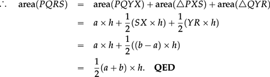
•that, if the parallel sides have lengths PQ = a and SR = b, and the perpendicular height is h, then the area of the shape can be found by dropping two perpendiculars, from P meeting SR at X and from Q meeting SR at Y, to produce a rectangle PQYX and two right angled triangles PXS and QYR, whose areas can be combined (using addition or subtraction— depending on the shape of the trapezium) to find the area of PQRS.
This primitive method can later lead to a proof of the well-known formula—at least in the simplest cases.
Claim Suppose X and Y are “internal” to the line segment SR. Then
area(PQRS)=  (a + b) × h.
Proof Since PQYX is a rectangle, we know that: XY = PQ = a, and PX = QY = h, and that SX + YR = SR − XY = b − a.
3.3.2“Composite shapes” The simple-minded approach to trapezia (by reducing the problem of finding the area of the trapezium to that of a rectangle and two right angled triangles) illustrates the reference to “composite shapes” in the second requirement. The kinds of combinations that are relevant here are very restricted, but they lie at the heart of all work with length, area, and volume.
•We calculate more complicated lengths (such as the perimeter of a polygon) by breaking them up into, or approximating them in terms of, combinations of line segments (or “one dimensional rectangles”).
•We calculate the area of more complicated shapes in 2D by breaking them up into, or approximating them in terms of, combinations of rectangles.
•We calculate the volume of more complicated shapes in 3D by breaking them into, or approximating them in terms of, combinations of cuboids (or “three-dimensional rectangles”).
In one dimension one may fudge the idea of “length” for the circumference of a circle by imagining a string wrapped round the circle, which is then “straightened out and measured”. This is fine—both as a way of conveying what we mean by the “circumference”, and to obtain a physical approximation. But it is not a mathematical method: the string is a physical object; the result is approximate—with no control over the error; and there is no way to be sure that the string does not change its length as one “straightens it out”. However, the most serious objection is that the idea does not extend to 2D and 3D. For example, one cannot take a curved 2D shape like a circular disc, cut it up and rearrange the pieces exactly to find its exact area; and one cannot take a curved surface, like the surface of an orange and “straighten it out, or lay it flat” to find its surface area. The idea that can be made to work in all dimensions is to concentrate on approximating more complicated shapes by “rectangles” (line segments, 2D rectangles, cuboids, etc.).
It is true that in two dimensions we often dissect polygons and other shapes into triangles rather than rectangles. But this trick has to be interpreted carefully. When we move from 2D to 3D, there is no way to extend the idea of a “triangle” as a way of making sense of “calculating volumes”: for there is no elementary way of finding the volume of a pyramid or tetrahedron. So we are free to use triangles in 2D, but we should think of each triangle as “half a rectangle” (on the same base, and with the same height), since the idea that works in all dimensions is to approximate shapes in terms of “n-dimensional rectangles”. That is,
•the basic building blocks for length are line segments (one dimensional rectangles);
•the basic building blocks for area are rectangles (two dimensional rectangles);
•the basic building blocks for volume are cuboids (three dimensional rectangles).
We also use composite shapes to approximate more awkward figures.
•The circumference of a circle is approximated by the perimeter of an inscribed or a circumscribed regular n-gon.
•The area of a circle is approximated from below by counting the number of unit squares inside it, and from above by counting the number of unit squares needed to just cover it.
3.3.3Understanding first, formulae second We repeat: pupils should be discouraged from using formulae ab initio. Instead they should be encouraged to imagine each “perimeter” as a sequence of separate line segments, and each “area” as being made up from, or approximated by, rectangles, or triangles (or a combination of both). In particular, they should use their common sense in working from the very beginning with composite shapes made from line segments, or from rectangles (or triangles), or from cuboids (or “wedges” as “half cuboids”). This helps to strengthen pupils’ basic understanding, since such composite shapes admit no general formula.
The extent to which pupils do not at present use their common sense in such matters is indicated by the following Year 9 items from TIMSS 2011.
3.3.3A The perimeter of a square is 36cm. What is the area of the square?
A 81cm2B 36cm2C 24cm2D 18cm2
3.3.3B The area of a square is 144cm2. What is the perimeter of the square?
A 12cmB 48cmC 288cmD 576cm
These are multiple choice items—so pupils were not required to calculate the answers. The false options here are either hard to obtain, or reflect severe mental sloppiness. So the results should provide serious food for thought (and not only in England).
3.3.3A Russia 62%,Hungary 55%,Australia 54%,USA 53%,England 51%
3.3.3B Russia 62%,Hungary 49%,Australia 48%,England 47%,USA 46%
3.3.4LengthThere is more to Section 3.3.2 than may appear: in simple language, it incorporates a definition of what we mean by “length”, of what we mean by “area”, and of what we mean by “volume”.
Pupils should understand the “perimeter of a rectangle” not via a formula, but using the common sense fact that it is made up of four line segments, whose lengths add up to give the perimeter (see examples 3.3.3A and 3.3.3B). The same idea applies to any polygon—where the perimeter is made up of a finite number of line segments, whose lengths can be added to give the perimeter of the polygon.
However, at first it is completely unclear how to extend this idea to measure the lengths of curves—such as the circumference of a circle of radius r. The physical idea of “the circumference of a circular, or cylindrical, lamp post” may be adequately captured by a piece of string that can be wound round the post and then straightened out and measured. But mathematics cannot depend on string. To capture the “length of a circular arc” mathematically we need
•to approximate it by a succession of line segments (such as the perimeter of a regular n-gon inscribed in, or circumscribed around, the circle), and
•then to realise that, as the number n of sides increases, the perimeter of the polygon gets closer and closer to the circle itself.
The cases which can be calculated easily, exactly, and instructively, without using trigonometry are:
n = 3: Pythagoras’ Theorem gives
“perimeter of inscribed regular 3-gon” = 3r.
n = 4: Pythagoras’ Theorem gives
“perimeter of inscribed regular 4-gon” = 4r .
.
n = 6: simple geometry gives
“perimeter of inscribed regular 6-gon” = 6r.
n = 8: Pythagoras’ Theorem gives
“perimeter of inscribed regular 8-gon” = 8r .
.
An inscribed regular octagon is still a long way from the circle itself, but we can see that the circumference of a circle of radius r is approximated ever more closely from below by the sequence

… < “circumference C of circle of radius r”.
The required circumference C of a circle would seem to be “some multiple of the radius r”, and the mysterious multiplier “ ” satisfies
5.1961… < 5.6568… < 6 < 6.1229… < … < .
The multiplier “” can also be bounded from above by considering circumscribed regular n-gons:
n = 3: Pythagoras’ Theorem gives
“perimeter of circumscribed regular 3-gon” = 6r.
n = 4: Pythagoras’ Theorem gives
“perimeter of circumscribed regular 4-gon” = 8r.
n = 6: simple geometry gives
“perimeter of circumscribed regular 6-gon” = 4r.
n = 8: Pythagoras’ Theorem gives
“perimeter of circumscribed regular 8-gon” = 16r( − 1).
Hence
5.1961… < 5.6568… < 6 < 6.1229… < … < < …
… < 6.6274… <6.9282… < 8 < 10.3922.
The mysterious multiplier “” is clearly somewhere around 6.3. Once we give it a name “2π”, and declare its actual value, we have the formula “C = 2πr” for the full circumference of a circle of radius r. We can then extend this to find the length of a semi-circle of radius r (πr), or of a quadrant  , or of the length of a circular arc of radius r with angle θ the centre.
One can then pose lots of moderately challenging problems to find the perimeters of composite shapes which are made entirely of rectangles (such as staircase-shaped figures), or which combine rectangles and circular arcs (such as a “running track”, or shapes made of rectangles and quadrants—both protruding and indented).
3.3.5Area We make sense of “area” in much the same way.
•If we take the area of a unit square as “1”, an m by n rectangle is made up of m × n unit squares, and so has area mn (square units)
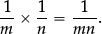
•We can break up the sides of the unit square into unit fractions, and conclude that mn copies of a  by
by  rectangle have total area 1, so that each has area
•A  by
by  rectangle can then be split into p × q rectangles each of which is by , and so has area
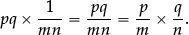
In short, the area of a rectangle with sides of lengths a units and b units can be shown to be equal to a × b square units for all possible values of a and b.
When we later come to consider “scaling” and “similarity”, the two facts:
•that the area of any rectangle is equal to “length × breadth”, and
•that the area of any more general shape is defined in terms of approximating the shape by combinations of rectangles
have an important hidden consequence. Whatever the area of a given shape may be, if we enlarge it (or “en-small” it) by multiplying all lengths by the same scale factor “r”, then the area of each and every approximating rectangle is multiplied by r2, so the area of the shape being approximated is multiplied by r2. So if one square has sides that are three times as long as another, then its area is nine times as large; and a circle of radius 4 has area 16 times as large as a circle of radius 1.
Long before we attempt a formal treatment of enlargement, or similarity, we need to build up the repertoire of basic results involving measures (as listed in the official requirements at the start of Section 3.3) using congruence. In particular, we need to connect the area of other plane figures to our fundamental shape—namely rectangles. And the most important of these “other figures” are parallelograms and triangles.
Suppose a parallelogram ABCD has longest diagonal AC. Let the perpendicular from A meet the line CD (extended) at X, and the perpendicular from C meet the line AB (extended) at Y. Then the parallelogram ABCD is completely enclosed in the rectangle AXCY, and the excess is formed by the two right angled triangles AXD and CYB—which fit together to make a smaller rectangle. Hence ABCD is equal to the difference between the large rectangle (with base XC and height XA) and the excess rectangle (with base XD and height XA)—whence:
Claim Area(parallelogram ABCD) = “base DC × height XA”.
Given any triangle ABC with “base AB”, we can draw the line through C parallel to the base AB, and the line through A parallel to the side BC. If these two lines meet at D, then ABCD is a parallelogram.
Claim ΔABC is congruent to ΔCDA
Proof ∠BAC = ∠DCA (alternate angles—see Part II, section 2.2.2.3)
AC = CA (same side)
∠BCA = ∠DAC (alternate angles)
∴ ΔABC is congruent to ΔCDA by the ASA congruence criterion. QED
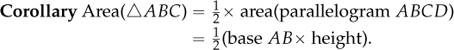
Pupils may think they already “know” the Corollary. What is new at Key Stage 3 is the idea that one can organise the vast lit of “known facts” in a way that identifies which are the “most basic” (namely congruence and the area of a rectangle), and how everything else can be derived from these basic results. Hence, one would like as many pupils as possible to appreciate
•that the result for the area of a triangle follows from
(i)congruence and
(ii)the result for the area of a parallelogram, and
•that the result for the area of a parallelogram follows from that for a rectangle.
In other words, we first highlight the congruence criterion, and then use it to reduce every question about the areas of other shapes (first parallelograms, then triangles, polygons, circles, etc.) to the basic question about the area of a rectangle. This is in some sense what we find in Book I of Euclid’s Elements (c. 300BC), where he goes on to show (in Proposition 47) the remarkable fact that this is all that is needed to prove Pythagoras’ Theorem.
Claim Let ΔABC be a right angled triangle with a right angle at C. Then the square ABPQ on the hypotenuse AB is equal to the sum of the squares CARS on side AC and BCTU on side BC.
Proof Let the perpendicular from C to AB meet AB at X and QP at Y.
It suffices to show that (half of) the square CARS is equal to (half of) the rectangle AXYQ.
AR is parallel to BS.
∴ ΔARC and ΔARB have the same base AR and the same height RS, so have the same area.
Also ΔARB ≡ ΔACQ (by SAS), so ΔARC and ΔACQ have the same area.
AQ is parallel to XY.
∴ ΔACQ and ΔAXQ have the same base AQ and the same height AX, so have the same area.
Hence ΔARC and ΔAXQ have equal area. QED
The proof needs to be acted out and expanded, but it has several advantages over most other proofs:
•It is very basic, in that it only uses congruence and the area of a triangle.
•It explains why the “square on the hypotenuse AB” is equal to a sum in a way that most proofs do not.
•The construction used is entirely natural: indeed, given a right angled triangle ABC with a right angle at C, the line CXY is the only way of splitting the “square on AB” into two parts that could possibly produce one part equal to the square on CA and the other equal to the square on CB.
In John Aubrey’s Brief lives (1694) we read of the philosopher Thomas Hobbes, that:
He was 40 years old before he looked on Geometry; which happened accidentally. Being in a Gentleman’s Library, Euclid’s Elements lay open, and ’twas the [Proposition] 47 [Book I]. He read the Proposition. By God, sayd he (he would now and then swear an emphaticall Oath by way of emphasis) this is impossible! So he reads the Demonstration of it, which referred him back to such a Proposition; which proposition he read. That referred him back to another, which he also read. [Continuing in this way, checking one thing after another] at last he was demonstratively convinced of that trueth. This made him in love with Geometry.
It is worth pondering on Hobbes’ scepticism and astonishment. Pythagoras’ Theorem is a completely unexpected result—and yet one that heralds much that lies ahead (from the Cosine rule, to scalar products, vector analysis, linear algebra, quadratic forms, and much, much more). One would like all pupils to recognise something of Hobbes’ surprise: Who would think of squaring lengths before adding?
Meantime, once we know how to calculate the area of a triangle, we can use this as required to calculate the area of any polygon by breaking it up into triangles and rectangles. For example, we saw in Section 3.3.1 that:
•if a trapezium ABCD has AB parallel to DC, then we can drop perpendiculars to break up the problem of finding the area of ABCD into that of finding the area of a rectangle and two right angled triangles;
•by cutting a regular n-gon into n congruent isosceles triangles we show later in the section that
area(regular n-gon with incircle of radius r) = (perimeter × radius r)
The area enclosed by any shape (including curved shapes such as a circular disc), is a measure of the “size” of the enclosed region. For a circle of radius r the exact value may prove elusive, but it can be approximated internally and externally to provide lower and upper bounds. For example, if we draw a circle of radius 5 centred at the origin (0, 0) on a square grid, the circle passes through the twelve grid points (± 5, 0), (0, ± 5), (± 3, ± 4), (± 4, ± 3). Counting unit squares inside the circle and those which just surround it then leads to the crude estimate
60 < area of circle of radius 5 < 88.
If we divide each unit in two and use squares of side , the circle with centre (0, 0) passes through (± 5, 0), (0, ± 5), (± 3, ± 4), (± 4, ± 3), with the points (±  , 0), (0, ± ) just inside the circle. Counting squares of size × leads to the slightly better estimate
69 < area of circle of radius 5 < 86.
However, merely counting smaller and smaller squares does not in itself suggest the crucial fact that the desired area is equal to a constant multiple of r2. For that we need something more systematic. There are two natural approaches to this: one is highly suggestive, but mathematically less precise; one is more precise and initially less suggestive (though ultimately suggestive in a different way).
The less precise (but more intuitive) approach is to cut the circular disc into 2n equal sectors, or “cake slices”, and arrange the pieces alternately pointing up and down, to form an “almost rectangle” with slightly sloping ends (each of length r—the radius) and slightly bumpy top and bottom edges (each of length equal to exactly half the perimeter of the circle—which we now know to be πr from Section 3.3.4). For larger and larger values of n—that is, for sectors with smaller and smaller angle  at the centre—the rearranged shape is more and more like a rectangle. This suggests that the total area of the circular disc is very close to that of an r by πr rectangle—namely r × πr = πr2.
The more precise approach is to consider regular n-gons inscribed in, and circumscribed around, a circle of radius r. One should start by carrying out the exact calculations for n = 4 and n = 6 as a concrete preliminary to the beautiful, and highly suggestive, general argument for regular n-gons that follows:
if n = 4:area(inscribed square) = 2r2 < area(circle radius r) < 4r2 = area(circumscribed square);
if n = 6:area(inscribed hexagon) =  area(circle) < 2 · r2 = area(circumscribed hexagon).
These calculations suggest that the area A of a circle of radius r is some “constant” multiple of r2, and that the mysterious constant satisfies
2 <  = 2.598… < constant < 3.464… = 2 < 4.
In general, if a regular polygon ABCDEFG… has an inscribed circle with centre O and radius r, then joining all vertices to the centre breaks up the polygon into n congruent isosceles triangles ABO, BCO, CDO, … . We know that
AB = BC = CD = …,
that the area of each triangle such as ABO is equal to
(base AB × height r),
and that the regular n-gon is equal to the sum of exactly n such triangles. Hence
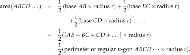
As the number n of sides increases, the regular n-gon approximates the circle more and more accurately and its area approaches the area of the circular disc.
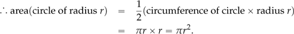
This links what we know about the circumference of a circle of radius r with the area of a circular disc of radius r, and shows that the mysterious “constant multiplier” is exactly π (that is, “half of the constant multiplier” 2π for the circumference of a circle).
Once the area of a circle of radius r is determined, one can pin down the area of a semicircle of radius r, of a quarter of a circle, and the area of a circular sector of radius r with angle θ at the centre. Pupils can then be asked to find the areas of all sorts of lovely composite shapes made from rectangles, triangles, and, circular sectors (both protruding and indented).
3.3.6Volume In one dimension there is really only one possible “shape”, namely a line segment. And the basic unit for “area” in 2D (namely the rectangle) is obtained by moving this 1D shape “perpendicular to itself in 2D”. Hence in 2D there is only one possible shape that results from moving a 1D figure (a line segment) perpendicular to itself—namely a rectangle. Our whole approach to area started by assuming that we know how to find the area of a rectangle. And the step from 1D to 2D was so short and sweet that we hardly noticed it.
But in 2D there are many different shapes, each of which can be moved “perpendicular to itself in 3D” to obtain a right prism with the given shape as base.
•Our basic unit of volume, the cuboid, is obtained by moving a rectangle perpendicular to itself in 3D to create a right prism with a rectangular base.
•We could just as easily start with a triangular base and move that perpendicular to itself.
•Or we could start with a regular polygon as base.
•Or we could start with a circle as base.
So there is much more initial work to be done before we begin to worry about how to find the volume of curved shapes— such as cones and spheres.
The first move is to establish the formula for the volume of a general cuboid. A cuboid with integer length sides can be built up by taking an integer number of unit cubes in each of the three directions. The formula can be extended to cuboids with fractional length sides in the same way that we extended the formula for the area of a rectangle. It follows that the volume of a general cuboid with sides of lengths a units, b units, and c units can be shown to be equal to a × b × c (cubic units) for all possible values of a, b and c giving the familiar formula:
volume(cuboid) = length × breadth × height.
Once this has result been established, the following sequence of steps allows us to calculate the volume of many other 3D shapes.
•First consider the cuboid as a right prism, (that is, as a three dimensional shape formed by moving the base rectangle at “right” angles to its plane) and interpret the formula for its volume as being
volume(right rectangular prism) = (area of base rectangle) × height.
•Then cut the base rectangle into two congruent right angled triangles, and so extend this formula to give the volume of a right prism with a right angled triangle as base (a “right triangular wedge”) as
volume(right prism with right triangular base)
= (area of base) × height.
•Then extend this formula to give the volume of any right prism with a parallelogram as base (surround the parallelogram by a rectangle, and hence surround the prism by a cuboid; then, just as in two dimensions, obtain the volume of the right prism by subtracting two “right triangular wedges” from the surrounding cuboid) to get:
volume(right prism with parallelogram base)
= (area of base parallelogram) × height.
•Then use the fact that any right triangular prism is half of a right prism with a parallelogram as base to show that its volume is given once more by:
volume(right prism with triangle as base)
= (area of base triangle) × height.
•We can then extend this same formula to any right prism with a polygon as base (by cutting up the base into triangles, and then adding up the volumes of the right triangular prisms):
volume of any right prism = (area of base figure) × height.
•Finally we extend this formula once more to a right circular cylinder (by approximating the base circle by regular polygons).
All these formulae can be explained and understood—and can then be used to find the volumes of an interesting variety of compound shapes. The formulae for the volumes of more complicated shapes (such as pyramids, cones, spheres) are more subtle, and are best delayed until Key Stage 4.
When we come to consider “scaling” and “similarity”, the two facts:
•that the volume of any cuboid is equal to
“(area of base) × height”,
or
“length × breadth × height”,
and
•that the volume of any more general shape in 3D is defined in terms of approximating them by combinations of cuboids (including “half cuboids”, or triangular wedges)
have a hidden consequence. Whatever the volume of a given shape may be, if we enlarge it (or “en-small” it) by multiplying all lengths by the same scale factor “r”, then the volume of each and every approximating cuboid is also multiplied by r3, so the volume of the shape being approximated is multiplied by r3. If one cube has sides that are three times as long as another, then its volume is 27 times as large; and a sphere of radius 4 has volume 64 times as large as a sphere of radius 1.
3.4.Constructions, conventions, and derivations
–use the standard conventions for labelling the sides and angles of triangle ABC, and know and use the criteria for congruence of triangles
–derive and use the standard ruler and compass constructions (perpendicular bisector of a line segment, constructing a perpendicular from/at a given point, bisecting an angle); recognise and use the perpendicular distance from a point to a line as the shortest distance to the line
–apply the properties of angles at a point, angles at a point on a straight line, vertically opposite angles
–apply […] triangle congruence […] to derive results about angles and sides […], and use known results to obtain simple proofs
–derive and illustrate properties of triangles, quadrilaterals, circles and other plane figures [for example, equal lengths and angles] using appropriate language and technologies
–understand and use the relationship between parallel lines and alternate and corresponding angles
–derive and use the sum of angles in a triangle and use it to deduce the angle sum in any polygon, and to derive properties of regular polygons
–apply angle facts, triangle congruence, similarity and properties of quadrilaterals to derive results about angles and sides, including Pythagoras’ Theorem, and use known results to obtain simple proofs
Congruence has already been introduced and used; and parallels have also featured (e.g. in parallelograms and trapezia). So this group of requirements, taken together, amounts to a relatively systematic “Euclidean” reorganisation of pupils’ geometrical knowledge and methods. But this “reorganisation” is not an end in itself. Once the three basic principles (congruence, parallels, similarity) have been clarified, once the backbone sequence of basic results has been established, and once the idea of only using previously proved results has been grasped, pupils gain access to what should be the main educational content of secondary school geometry—namely the wonderful world of accessible, yet elusive problems. To keep things relatively short, the exposition here focuses mainly on the underlying framework of basic results and methods which is needed to support this pupil activity. However, it is essential for teachers not only to grasp the underlying framework, but also to engage with the kinds of problems this framework opens up for pupils (and teachers) to enjoy. For a systematic development of deductive problems for mid-late Key Stage 3, we recommend the book Crossing the Bridge by G. Leversha (UKMT Publications 2008). Dedicated sets of problems can also be found in the series Extension Mathematics by Tony Gardiner (Oxford University Press 2007):
•Book Alpha: T5 (perimeters); T9, E2 (angles); T11, C7 (drawing conclusions); C17 (triangles); C19, E14 (areas and volumes)
•Book Beta: T11, T15 (drawing conclusions); C4, C7, C15 (congruence); T17, C11, E4 (angles); T20 (triangles); T26, C18 (areas and perimeters); C2 (parallel lines); C5 (ruler and compass constructions); C27 (volumes)
•Book Gamma: T10 (parallel lines); T17, C35 (Pythagoras’ Theorem); T24 (loci); T8, C8 (circles); C10 (angles in regular polygons); C15 (volumes and prisms); C3, C39 (miscellaneous problems).
After a brief general introduction (Section 3.4.1) we address the very first listed requirement in two parts (Sections 3.4.2 and 3.4.3). We then discuss the role of the standard “ruler and compass constructions” in Section 3.4.4, before focusing on angles, and deriving the simplest consequences of the congruence criteria (relating to isosceles triangles and regular polygons) in Section 3.4.5. Section 3.4.6 examines the consequences of the parallel criterion—in particular the sum of angles in a triangle and results relating to parallelograms. Finally Section 3.4.7 comments briefly on the requirements relating to similarity. (The two remaining official requirements under the heading of Geometry and measures are discussed briefly in Section 3.5.)
3.4.1Towards formal geometry As with all aspects of elementary mathematics, there is no “royal road” to success in geometry. The approaches adopted in England since the 1960s introduced all manner of delights, which one may hesitate to discard. But they have singularly failed to produce school leavers able to analyse configurations in two- and three-dimensions.
During this period a number of teachers and authors have continued to insist, and to demonstrate, that the most effective framework within which ordinary students can apprehend and ‘calculate exactly’ with geometrical information is that which analyses more complicated figures in terms of triangles. This is the thrust of the Euclidean framework illustrated by the sequence of official requirements listed at the start of Section 3.4.
Informal work at Key Stage 1 and Key Stage 2 to make sense of shapes and patterns in 2D and 3D prepares the ground for the ‘more formal’ treatment later in Key Stage 3 and at Key Stage 4. We have already stressed the need for structured work at Key Stage 2 and in early Key Stage 3 to include drawing and measuring (Section 3.2.1), calculating angles (described briefly in Part II, Section 2.3.5), and work with lengths, areas and volumes (Section 3.3.1). Such work develops the ideas and language that are needed when we begin to reorganise our approach to Euclidean geometry during Key Stage 3 (in terms of congruence, parallels, and similarity). The sequence of requirements listed at the start of Section 3.4 should be seen as ushering in this semi-formal phase.
The full thrust of formal Euclidean geometry only takes root late in Key Stage 3. And though the foundations are laid in Years 7 and 8, it is not surprising that most of the released Year 9 items from TIMSS 2011 focus on calculation and construction, rather than on deduction. However, one item is perhaps relevant.
3.4.1A [A convex pentagon labelled ABCDE is shown, including diagonals AC and AD.] What is the sum of all the interior angles of pentagon ABCDE? Show your work.
The dissection of the pentagon in the accompanying diagram into three triangles ABC, CAD, and DEA invites (but does not force) pupils to use the “known fact” that the angles in any triangle add to 180°. Since most Year 9 pupils have known this “fact” for several years, it seems reasonable to hope that significant numbers might manage to produce the answer of 540°, with an acceptable justification—even if expressed rather crudely as:
ΔABC + ΔACD + ΔADE = 180 + 180 + 180 = 540,
 ABCD + ΔADE = 360 + 180 = 540.
The reported results therefore underline the challenge of trying to get pupils to “reason geometrically”. The mark scheme awarded 2 points for an acceptable solution (including a justification), with 1 point for the numerically correct answer, but with an incorrect reason (and maybe for an acceptable reason, with an incorrect answer). We give the percentage of pupils scoring 2 points (with the percentage scoring at least 1 point in brackets):
3.4.1A Hungary 22% (29);Russia 19% (35);England 17% (20);Australia 13% (19);USA 12% (16)
It is probably worth noting three additional results from the Far East. The Japanese scores of 72% (and 81%) show that it is possible to do considerably better than we do at present. At the same time the Singapore scores of 55% (and 60%), and the Hong Kong scores of 38% (and 51%), suggest that it would be rash to expect too much, too soon, from too many pupils.
3.4.2Conventions The details relating to the first half of the first listed requirement were explored at length in Part II, Section 2.2.2.3, namely for pupils to learn
–to use the standard conventions for labelling the sides and angles of triangle ABC.
These conventions establish the language and grammar of all “geometrical calculation”.
Mathematics in general succeeds by translating sense impressions, and language or sounds, into symbols which allow exact calculation. For example, we replace “words for numbers” by numerals and place value, which then makes it possible to develop exact methods for “numerical calculation”. Similarly, it is only when general relations are expressed as algebraic expressions that we have a chance of making deductions we might otherwise overlook. For example, as long as the problem
“Find a prime number that is one less than a square”
is presented in non-mathematical language, its analysis remains elusive. But as soon as it we translate this into the appropriate mathematical language:
“When is n2 − 1 prime?”
we immediately have the chance of seeing how to proceed by engaging in “algebraic calculation”, since “n2 − 1” should trigger the well-known factorisation
n2 − 1 = (n − 1)(n + 1),
so n2 − 1 can only be prime if n − 1 = 1.
In the same spirit, the English words “triangle” or “quadrilateral” conjure up a visual impression, or imagined shape. But one cannot calculate with such a visual impression. If we wish to refer to, and to calculate with, a particular triangle or quadrilateral, we need to give it a name in accordance with certain conventions.
The labelling conventions are chosen to communicate reliably between individuals, and to reflect the geometric structure of the object being labelled. Points are routinely denoted by capital letters (preferably italic). Two points A, B determine a line AB. But in England we use the same notation for the line segment which starts at A, runs to B, and then stops. And we use the same notation again for the length of the line segment! In other countries, these three different ideas are given different notations. It is unclear who has the power to change this confusion. But it is completely clear that, as long as we continue to use “AB” to denote all three ideas, it is essential for teachers to make sure that the associated language used in the classroom and in pupils’ written solutions always makes it clear which meaning is intended.
A polygon is a “broken” (or bent) sequence of line segments. Hence, when labelling a polygon, the sequence in which the vertices are named matters. A quadrilateral ABCD has to be labelled in cyclic order, where the edges are the successive line segments, or edges, that make up the quadrilateral: with edges AB and BC (meeting at the vertex B), BC and CD (meeting at vertex C), CD and DA (meeting at vertex D), and DA and AB (meeting at vertex A).
The whole of geometry in 2D and in 3D rests on the discovery that triangles hold the key to the construction and analysis of more complicated shapes. When we label the vertices of a triangle ΔABC, the cyclic order is not a problem: because there are only three vertices, the only choice is to list the vertices in clockwise, or in anticlockwise order. Each of the three vertices gives rise to an (internal) angle:
∠ABC (often abbreviated as “∠B”, or just “B”), ∠BCA (abbreviated as “∠C”, or “C”), and ∠CAB (abbreviated as “∠A”, or “A”).
And the length of each side of the triangle is conventionally labelled with the lower case version of the opposite vertex:
side AB (opposite vertex C) has length c, side BC has length a, side CA has length b.
More awkward is the fact that whenever push comes to shove, a ‘triangle’ is not just a three-cornered shape: it is a labelled, or ordered, triple ABC, where the order matters. If one only knows the three vertices, but not the order, then this corresponds to several different triangles: the triangles ΔABC, ΔBCA, ΔCAB, ΔBAC, … are in some sense different (as becomes clear when aligning triangles to demonstrate congruence—see Section 3.4.3). Even if we choose not to insist on such precision all the time, whenever we come to do some kind of calculation with a triangle, or a quadrilateral, we find that the order matters.
In a similar spirit, Key Stage 3 should witness a marked shift in how geometric objects are defined.
•In primary school, an object is pinned down (or “apprehended”) by accumulating an ever-increasing list of “properties” (so that a “rectangle” is understood through all its properties: opposite pairs of sides equal and parallel, four right angles, equal diagonals which bisect each other, and so on).
•In Key Stage 3 this “encyclopedic” approach to the question “What is a rectangle?” should be replaced by the idea of a definition as a minimal specification. Hence
–a “rectangle” is defined to be “a parallelogram with one right angle”;
–a “parallelogram” is defined to be “a quadrilateral with opposite pairs of sides parallel”; and
–a “right angle” is defined to be “half a straight angle”.
This not only makes it clear what exactly we mean by a “rectangle”, it also makes it much easier to check that a given quadrilateral is in fact a rectangle (since we only have to check (a) that it is a parallelogram, and (b) that it has at least one right angle). Once we have done this, we know that every other property of a rectangle comes for free—without the need to check.
3.4.3Congruence The second half of the first listed requirement, namely
–to know and use the criteria for congruence of triangles
was explored in Section 3.2.3 above and in Part II, Section 2.2.2.3. Further consequences arise in Section 3.4.4, 3.4.5, and 3.4.6 below.
Two (ordered) triangles ΔABC and ΔDEF are congruent if the (ordered) correspondence
matches up each of the six ingredients of triangle ΔABC with those of triangle ΔDEF in such a way that
•all three corresponding pairs of line segments are equal:
AB = DE, BC = EF, CA = FD,
and
•all three corresponding pairs of angles are equal:
∠A = ∠D, ∠B = ∠E, ∠C = ∠F.
We write this as:ΔABC ≡ ΔDEF (which we read as “triangle ABC is congruent to triangle DEF”).
“Congruence of triangles” only makes sense between ordered triangles. And it can help pupils to see more clearly which vertex of the first triangle corresponds to which in the second triangle, and which side of the first triangle corresponds to which in the second triangle if pupils initially write
ΔABC
≡ ΔDEF
lining up corresponding vertices and edges vertically over each other (as with column arithmetic):
•with vertex A directly above vertex D, B directly above E, C directly above F, and
•with edge AB directly above edge DE, BC directly above EF, CA directly above FD.
The three basic congruence criteria (SSS, SAS, and ASA) arise naturally from drawing and construction exercises, and the SSS-congruence criterion plays a significant role in the next Section 3.4.4 to show that the standard ruler and compass constructions do what they claim:
triangles ΔABC and ΔDEF are congruent (by SSS) if AB = DE, BC = EF, and CA = FD;
triangles ΔABC and ΔDEF are congruent (by SAS) if AB = DE, ∠BAC = ∠EDF, and AC = DF;
triangles ΔABC and ΔDEF are congruent (by ASA) if ∠BAC = ∠EDF, AB = DE, and ∠ABC = ∠DEF.
The RHS congruence criterion is not part of this basic congruence criterion, so does not really belong at this stage. It arises as the degenerate instance of the failed ASS criterion (where the angle “A” in “ASS” is a right angle, and so is neither acute nor obtuse). The fact that RHS guarantees congruence depends on Pythagoras’ Theorem, since knowing two sides and a right angle then determines the third side. So RHS is a special case of SSS.
3.4.4Congruence and ruler and compass constructions “Construction” at Key Stage 3 takes on a slightly different meaning, moving
•from measuring work with rulers and protractors at Key Stage 2 and early Key Stage 3
•to a simple, hands-on, geometrical framework using “ruler and compasses”, which avoids measuring altogether, in which the familiar “measuring ruler” becomes a straightedge (that is, a mere straight-line-drawer), and the focus switches from measuring lengths to “equality” of line segments (e.g. as radii of a given circle, created by a pair of compasses).
We stick to the tradition of referring to these latter constructions as ruler and compass constructions—even though the ruler is being used as an “ideal” mental straightedge (and its crude, approximate markings play no role).
•Given two points A and B, the “ruler” is simply a way of physically capturing the idea that one can imagine the line or line segment “AB” determined by these two points; and
•given a point O (as centre) and another point P, the “compasses” are a way of physically capturing the “ideal” construction of the circle with centre O and passing through P.
That is, the two instruments are in some sense not being used to perform actual constructions, but to illustrate imagined ideal constructions (performed with ‘heavenly’ straightedge and compasses).
Ruler and compass constructions offer a natural psycho-kinetic embodiment of the simplest parts of formal geometry (for example, allowing pupils to experience SSS-congruence directly). The constructions themselves are experienced directly; and the proofs that the basic constructions do what they claim constitute an introduction to the subsequent transition from physical to formal geometry. Hence ruler and compass constructions embody four rather different aspects of secondary mathematics.
•The first is the clean simplicity of the basic moves:
–to construct the line AB through two known points A and B,
–to construct the circle with known centre A passing through a known point B, and
–to obtain “new known points” as the points of intersection of two constructed lines, or of a constructed line and a circle, or of two constructed circles.
•The second aspect is the act of drawing itself (which may at first be ungainly, but which benefits hugely from practice, which exploits the links between hand, eye, and brain, gives physical substance to geometrical ideas, and leads ultimately to quiet satisfaction after a well-implemented construction).
•The third aspect is to imagine the act of drawing without first carrying out each construction, so that one can begin to combine standard constructions as basic moves in a chain that achieves some more complicated goal: (for example, we can imagine how one might use ruler and compasses to construct an equilateral triangle—or a square, or a regular pentagon, or a regular hexagon, or a regular octagon—inscribed in a circle with centre at O and passing through the point A).
•The fourth aspect is the simple deductive structure, based mainly on the SSS-congruence criterion, that shows how “equal lengths” (which is all one can create using compasses, where two radii of the same circle are necessarily equal) leads to congruence, and hence forces certain angles to be equal.
The idea that mathematical objects need to be “constructed”, rather than “postulated” or plucked out of thin air, lay at the heart of ancient Greek mathematics. The assumptions which underlie ruler and compass constructions were declared as the first three of their five “axioms” or principles:
•to construct a line segment AB joining two known points A, B;
•to extend this line segment as far as one wishes in either direction;
•to construct the circle with known centre O and passing through a known point A.
Many of the results they proved were presented as constructions. For example, the very first Proposition in Book I of Euclid’s Elements:
“On a given finite straight line [segment AB] to construct an equilateral triangle [ABC].”
Construction: Draw the circle with centre A passing through B, and the circle with centre B passing through A. Let these two circles meet at C and at D.
∴ AB = AC (radii of the same circle) and BA = BC (radii of the same circle).
∴ ΔABC is equilateral. QEF
Genuine proofs ended with a statement (in Greek)
“which is that which was to be proved”.
This is rendered in Latin as “Quod Erat Demonstrandum” and abbreviated as “QED”. In contrast, constructions like the one above ended with the statement
“being what it was required to do”,
which is rendered in Latin as “Quod Erat Faciendum” and abbreviated as “QEF”.
This may all seem to have little to do with school mathematics. But it is worth reflecting on the links between this “constructive” approach to mathematical concepts and the psychology of the learner. As mathematics became more abstruse in the eighteenth, nineteenth, and early twentieth centuries, its ideas and methods were increasingly postulated abstractly. This approach proved exceedingly powerful; but it also made the subject less accessible, and led to philosophical difficulties. The advent of computers has reminded us afresh of the need to be able to construct the ideas about which we reason in mathematics: knowing that a curve crosses the x-axis and so has a “root” is one thing; but we also need effective methods for finding that root. Something analogous applies to learners, where a constructive approach often allows a more meaningful kind of engagement than a purely logical analysis. (This observation also seems to have been behind John Perry’s proposed reforms in the early 1900s.)
The official requirement that pupils should
–derive and use the standard ruler and compass constructions (perpendicular bisector of a line segment, constructing a perpendicular from/at a given point, bisecting an angle); recognise and use the perpendicular distance from a point to a line as the shortest distance to the line
encourages this kind of healthy, constructive engagement, and does so using “ruler and compasses” in a way that is consistent with the Euclidean reworking of geometry. It is therefore to be welcomed (though, as we shall see, the final reference to “shortest distance to the line” is slightly out of place).
The first “standard construction” is implicit in Euclid’s Proposition 1.
To construct the perpendicular bisector of a given line segment AB.
Construction: Draw the circle with centre A passing through B, and the circle with centre B passing through A. Let these two circles meet at C and at D.
We may not yet know how to construct the midpoint of the line segment AB; but the midpoint certainly exists, so let us “imagine” it (somewhere between A and B) and give it a name, M.
We claim that ΔCMA ≡ ΔCMB (by SSS).
∴ ∠CMA = ∠CMB, so each angle is half a straight angle, and CM is perpendicular to AB.
Similarly, DM is perpendicular to AB.
∴ CMD is a straight line, so the line CD crosses AB at its midpoint M.
∴ CD is the required perpendicular bisector. QEF
The second standard construction uses the same idea.
Given a line segment AB and a point P, to construct the perpendicular from P to AB.
Construction:
(i) Suppose first that P lies on the line AB.
Clearly P cannot be the same point as both A and B. So we may suppose that P ≠ B.
Draw the circle with centre P passing through B, and let it meet the line AB (= BP) again at C.
Then P is the midpoint of BC.
Use the first standard construction to find the perpendicular bisector of BC, and this will be the perpendicular to AB at the point P.
(ii) Suppose next that P does not lie on the line AB.
By drawing the circles with centre P passing through A and through B we can choose the point furthest from P—which we may suppose is B.
Draw the circle with centre P passing through B, and let it meet the line AB again at C. (The point C lies on the line AB, but is not internal to the line segment AB.)
Use the first standard construction to find the midpoint M of BC.
∴ ΔPMB ≡ ΔPMC (by SSS)
∴ ∠PMB = ∠PMC, so each is half a straight angle.
∴ PM is the perpendicular from P to AB. QEF
The third standard construction is slightly different. Because ruler and compasses can only make lengths equal, it again uses SSS-congruence—this time to conclude that two angles are equal.
Given two lines BA and BC meeting at the point B, to construct the bisector of ∠ABC.
Construction: Draw the circle with centre B passing through C and let this circle meet the segment BA (extended if necessary beyond the point A) at D.
∴ BC = BD (radii of same circle)
Draw the circle with centre C passing through B, and the circle with centre D passing through B, and let these two circles meet at B and again at E.
∴ CB = CE (radii of same circle) and DB = DE (radii of same circle).
∴ ΔCBE ≡ ΔDBE (by SSS)
∴ ∠CBE = ∠DBE, so the line BE bisects ∠ABC. QEF
There are lots of lovely problems which exploit these three basic constructions. Once we are in a position to use “equal alternate (or corresponding) angles” as a criterion for two lines to be parallel, we can extend the second standard construction to obtain the line through P parallel to AB.
Given a line AB and a point P not on AB, to construct the line through P parallel to AB.
Construction: Construct the perpendicular from P to AB, meeting AB at the point X.
Then construct the perpendicular PY to PX at the point P.
The fact that ∠AXP and ∠XPY are right angles, then implies that PY is parallel to AB. QEF
We can also explore the question of constructing regular polygons. The flower petal construction described in Section 3.2.1 shows how to construct a regular hexagon ABCDEF inscribed in a given circle with centre O and passing through A. By taking every second vertex, we obtain a way of constructing an equilateral triangle ACE inscribed in the circle with centre O.
The question as to which other regular polygons can be constructed in this way was addressed (and answered completely) by Carl Friedrich Gauss in his late teens in the mid-late 1790s, and published in his famous book Disquisitiones arithmeticae, 1801 (at the time, Latin was still the main international language for communicating scientific results). To construct a square, let AO meet the circle again at C, construct the perpendicular bisector of the line segment AC, and let this meet the circle at B and at D; then one can prove that ABCD is a square. One can also find relatively simple ways of constructing a regular pentagon in the circle with centre O (though proving that they really work may have to wait until Key Stage 4). And once we know how to construct a regular 4-gon ACEG in the circle with centre O passing through A, we can use the first standard construction to construct the perpendicular bisector of each side and so find the points B, D, F, H where these perpendicular bisectors cut the circle—thus constructing a regular 8-gon ABCDEFGH. Similarly, once we know how to construct a regular 5-gon, we can construct a regular 10-gon. But it is impossible to construct a regular 7-gon, or a regular 9-gon, or a regular 11-gon with ruler and compasses.
The final requirement for pupils to:
recognise and use the perpendicular distance from a point to a line as the shortest distance to the line
is slightly out of place here. We saw how to construct the perpendicular from a point P to meet AB at the point X. But it is not obvious that PX is the shortest distance from P to AB. (The easiest way to see this is to consider any other point Y on the line AB and then to apply Pythagoras’ Theorem to the right angled triangle PXY to see that PY is greater than PX.)
3.4.5The basic consequences of congruence The simplest geometrical result of all is that “vertically opposite angles are always equal” as required by
–apply the properties of angles at a point, angles at a point on a straight line, vertically opposite angles.
Claim Whenever two lines cross at a point P, any pair of vertically opposite angles A and A′ at P are necessarily equal.
Proof: Let B be the angle “between” the two vertically opposite angles A and A′ at P.
Then A + B is the straight angle on one line, and B + A′ is the straight angle on the other line.
∴ A + B = B + A′, so A = A′. QED
In general the size of an angle is defined in terms of fractions of a “straight angle” (the “angle” at a point P on a straight line). For example, if we bisect a straight angle, then each half is a right angle. Thanks to the ancient Babylonians, we still measure angles in degrees, with each straight angle equal to 180°, so each right angle is equal to 90°. We are not sure why they chose 360° for a full turn. However, it may be related in some way
(a)to their use of the sexagesimal numeral system (base 60), and
(b)to their use of angles in astronomy, and the connection between the apparent movement of the observed stars and what they took to be the number of days in a year.
The rest of this section focuses on the SSS, SAS, and ASA congruence criteria. These are in many ways more fundamental than the criterion for two lines to be parallel (which we address in Section 3.4.6), in that they apply to geometries where the parallel criterion fails—allowing us to show that certain angles, or line segments, are equal (as in Section 3.4.4, where we dropped perpendiculars, and where we bisected any given angle). The miracle of Euclidean geometry is how much more one can prove by combining these two principles.
We start by developing the “backbone” of results that depend only on congruence. This obliges us to interpret the two slightly confused official requirements:
–apply […] triangle congruence […] to derive results about angles and sides […], and use known results to obtain simple proofs
–derive and illustrate properties of triangles, quadrilaterals, circles and other plane figures [for example, equal lengths and angles] using appropriate language and technologies
The problem here is that the wording in the full requirement (including the parts which have here been omitted) confuses
•the experiential Key Stage 2 approach to geometry (where one “collects and uses facts” without any definitions or proofs) and
•the Key Stage 3 approach, which begins to organise geometrical knowledge through minimal definitions, respecting conventions, emphasising the three basic principles (the congruence criterion, the parallel criterion, and the similarity criterion), and deriving those “facts”, or “properties”, which are most useful.
If we disentangle this confusion, and focus on what should be the distinctive Key Stage 3 approach, then the first move has to be to prove the basic facts about isosceles triangles. A triangle ABC in which AB = AC is called isosceles, with base BC and with apex A. (“Iso” means “same” in Greek; and “sceles” means “legs”, or sides.)
Claim if AB = AC, then ∠ABC = ∠ACB (“the base angles of any isosceles triangle are equal”). Moreover, the line AM joining the apex A to the midpoint M of the base BC (the “median”) is also the perpendicular bisector of the base BC, and the bisector of the apex angle ∠BAC.
Proof Construct the midpoint M of the base BC.
Then ΔABM ≡ ΔACM (by SSS).
∴ ∠ABM = ∠ACM, so the two base angles ∠ABC and ∠ACB are equal.
Also ∠AMB = ∠AMC, so each is equal to half a straight angle—that is, a right angle.
And ∠BAM = ∠CAM, so AM bisects the angle ∠BAC. QED
Claim If ∠ABC = ∠ACB, then AB = AC (“if the base angles are equal, the triangle is isosceles”).
∴ AB = AC. QED
Claim (a) If M is the midpoint of BC, and MX is perpendicular to BC, then XB = XC. That is, each point on the perpendicular bisector of BC is equidistant from B and from C.
(b) Conversely, if Y is equidistant from B and from C, then Y lies on the perpendicular bisector of BC.
Hence the perpendicular bisector of a line segment BC is precisely the locus of all points that are equidistant from B and from C.
Proof (a) ΔXMB ≡ ΔXMC (by SAS, since XM = XM, ∠XMB = ∠XMC, MB = MC).
∴ XB = XC.
(b) Join YM. Then ΔYMB ≡ ΔYMC (by SSS).
∴ ∠YMB = ∠YMC, so each is half of a straight angle. QED
Isosceles triangles arise naturally when working with circles: if A and B lie on the circle with centre O, then OA = OB, so ΔOAB is isosceles. Hence the perpendicular from O to AB bisects the base AB and also bisects the angle ∠AOB. Isosceles triangles also feature in the following useful result.
Claim A regular n-gon ABCDEF… has a centre O, and is inscribed in a circle with centre O.
Proof Let the perpendicular bisector of AB meet the perpendicular bisector of BC at O. By a previous result, OA = OB, and OB = OC. Hence OA = OC and the circle with centre O passing through A, also passes through B and C. We show that this circle necessarily passes through the vertex D, and hence through all vertices of the regular polygon.
∴ ΔOAB is isosceles, so ∠OAB = ∠OBA, and ΔOBC is isosceles, so ∠OBC = ∠OCB.
Moreover ΔOAB ≡ ΔOBC (by SSS: since OA = OB, OB = OC, and AB = BC).
∠OAB = ∠OBA = ∠OBC = ∠OCB = (∠ABC).
∴ ∠OCD = ∠BCD − ∠OCB = (∠ABC) = ∠OBC.
∴ ΔOBC ≡ ΔOCD (by SAS: OB = OC, ∠OBC = ∠OCD, BC = CD).
∴ OC (in ΔOBC) = OD (in ΔOCD) so the circle with centre O passing through A also passes through D.
Continuing in this way shows that the circle passes through every vertex of the regular polygon. QED
3.4.6The parallel criterion and angles in a triangle To prove more interesting results—such as to
–derive and use the sum of angles in a triangle and use it to deduce the angle sum in any polygon
we need more than just the congruence criterion. In particular, we need to
–understand and use the relationship between parallel lines and alternate and corresponding angles.
This is the second organising principle in geometry—namely the criterion for two lines in the plane to be parallel. Given any two lines in the plane, a transversal is a third line that cuts both of the two given lines. The parallel criterion declares that:
•two lines are parallel precisely when the alternate angles (or the corresponding angles) created by a transversal are equal.
This is a rather subtle criterion, but one which can be made thoroughly plausible.
The formal proof that the three angles in any triangle ABC add to a straight angle echoes the primary school activity of tearing off the three corners and fitting the pieces together crudely against a ruler. But here we use “God’s ruler” (namely the line through C parallel to AB), and we fit the three angles together perfectly and in a very particular order (∠A + ∠C + ∠B).
Claim The three angles in any triangle ΔABC add to a straight angle.
Proof Construct the line XCY through C parallel to AB (with X on the same side of CB as A).
Then ∠XCA = ∠BAC = ∠A (alternate angles)
and ∠YCB = ∠ABC = ∠B (alternate angles).
∴ ∠A + ∠C + ∠B = ∠XCA + ∠ACB + ∠YCB. QED
A quadrilateral ABCD can be split into two triangles (by drawing one of the diagonals AC, BD), so the sum of the four angles in any quadrilateral is “2 × 180°”. The same idea shows that the angles in any polygon with n sides have sum (n − 2) × 180°. These simple observations open the door to hundreds of wonderful (non-obvious, multi-step) problems involving angle chasing (see, for example, Extension mathematics, Tony Gardiner: Book Alpha, Sections T9, E2; and Book Beta, Sections T17, C11, E4).
The last seven words of the requirement
–derive and use the sum of angles in a triangle and use it to deduce the angle sum in any polygon, and to derive properties of regular polygons
are slightly out of place here. A regular polygon is defined to be a polygon whose sides are all equal and whose angles are all equal. It should be a major focus of secondary geometry to explore the geometry of regular polygons—at least including regular 3-gons, regular 4-gons, regular 5-gons, regular 6-gons, and regular 8-gons. And whilst it follows from the above that each angle in a regular n-gon is equal to
almost anything else one might prove about regular polygons depends on the congruence criteria (in particular, properties of “isosceles triangles”). This observation even applies to proving that certain diagonals and sides are parallel.
Claim Let ABCDE be a regular pentagon. Then each diagonal is parallel to the opposite side.
Proof We show that AC is parallel to ED.
∠ABC = (1− ) × 180° = 108°.
BA = BC, so ΔBAC is isosceles. Hence ∠BAC = ∠BCA = 36°.
∴ ∠CAE = 72°, so ∠CAE + ∠DEA = 180° whence AC is parallel to ED. QED
The most important application of the basic property of parallel lines is to derive results about parallelograms. A parallelogram is a quadrilateral ABCD in which opposite pairs of sides AB, DC and BC, AD are parallel. Most results relating to parallelograms depend on the congruence criteria. But two results depend only on the basic property of parallel lines.
Claim If ABCD is a parallelogram, then opposite angles are equal: ∠A = ∠C, ∠B = ∠D.
Conversely, if ABCD is a quadrilateral with ∠A = ∠C, ∠B = ∠D, then ABCD is a parallelogram.
Proof Suppose ABCD is a parallelogram. Then AB is parallel to DC, so ∠A + ∠D = 180°.
And AD is parallel to BC, so ∠D + ∠C = 180°.
∴ ∠A = ∠C, and ∠B = 180° − ∠A = 180° − ∠C = ∠D.
Conversely, suppose ABCD is any quadrilateral in which opposite angles are equal in pairs: ∠A = ∠C, ∠B = ∠D. Since
∠A + ∠B + ∠C + ∠D = 360°,
it follows that ∠A + ∠B = 180°, so AD is parallel to BC. Similarly ∠B + ∠C = 180°, so AB is parallel to DC. QED
A rectangle is defined to be “a parallelogram with (at least one) right angle”. If the rectangle is ABCD, and if the right angle is at A, then from the above result it follows that ∠C is also a right angle. Hence ∠B + ∠D = 180°; since ∠B = ∠D, it follows that ∠B and ∠D are also right angles. However, there is no simple way to conclude that “opposite sides of a rectangle are equal” other than by proving the result for parallelograms in general (using ASA-congruence).
Claim If ABCD is a parallelogram, then opposite sides are equal in pairs: AB = DC and BC = AD.
Proof Draw the diagonal AC.
∴ ∠BAC = ∠DCA (alternate angles)
AC = CA
∠BCA = ∠DAC (alternate angles)
∴ ΔBAC ≡ ΔDCA (by ASA)
∴ BA = DC and BC = DA. QED
Claim If ABCD is a rectangle, then AC = BD.
Proof We claim that ΔABC ≡ ΔBAD (by SAS: since AB = BA, ∠ABC = ∠BAD = 90°, and BC = AD (opposite sides of parallelogram)).
∴ AC = BD. QED
Each result one can prove for parallelograms has a converse which (if true) should also be proved, since it allows us to identify a parallelogram on the basis of other characteristic properties.
Claim If ABCD is a quadrilateral in which AB = DC and BC = AD, then ABCD is a parallelogram.
Proof Draw the diagonal AC.
∴ ΔBAC ≡ ΔDCA (by SSS).
∴ ∠BAC = ∠DCA, so AB is parallel to DC (alternate angles equal), and ∠BCA = ∠DAC, so BC is parallel to AD (alternate angles equal). QED
Claim If ABCD is a parallelogram, then the diagonals AC and BD bisect each other.
Conversely, any quadrilateral ABCD whose diagonals bisect each other is a parallelogram.
Proof Let the two diagonals meet at X.
∴ ∠ADX = ∠CBX (alternate angles)
DA = BC (opposite sides of a parallelogram)
∠DAX = ∠BCX (alternate angles).
∴ ΔADX ≡ ΔCBX (by ASA)
∴ DX = BX and AX = CX, so the diagonals bisect each other.
Now let ABCD be any quadrilateral whose diagonals AC, BD bisect each other at X.
Then AX = CX and DX = BX, and ∠AXD = ∠CXB (vertically opposite angles).
∴ ΔADX ≡ ΔCBX (by SAS).
∴ ∠DAX = ∠BCX, so DA is parallel to CB (alternate angles equal), and
Similarly we can show that ΔABX ≡ ΔCDX (by SAS).
Hence ∠BAX = ∠DCX, so AB is parallel to DC (alternate angles equal). QED
A rhombus is a parallelogram ABCD with adjacent sides equal; AB = AD. And a square is a rhombus which is also a rectangle.
Claim The two diagonals of a rhombus ABCD are perpendicular.
Proof Let the two diagonals meet at X. Then DX = BX so ΔAXD ≡ ΔAXB (by SSS).
∴ ∠AXD = ∠AXB. QED
In a rhombus ABCD, each diagonal splits the rhombus into two isosceles triangles. Hence other properties of a rhombus (and their converses) tend to exploit the basic property of isosceles triangles (and its converse).
–identify and construct congruent triangles, and similar shapes by enlargement, with and without coordinate grids
–apply angle facts, triangle congruence, similarity and properties of quadrilaterals to derive results about angles and sides, including Pythagoras’ Theorem, and use known results to obtain simple proofs
–use Pythagoras’ Theorem and trigonometric ratios in similar triangles to solve problems involving right angled triangles
The first two requirements have both been addressed elsewhere (in Section 3.2 and 3.2.3, and in Section 3.4.5 respectively). They are linked here because both mention “similar shapes” or “similarity”, and this idea has to be addressed to prepare the way for simple trigonometry (as in the third listed requirement).
We noted in Section 3.2 that the reference to “similar shapes” in the first of the above requirements is largely “informal”, and that the initial emphasis here should be practical. The formal notion of similarity should emerge from pupils’ own experience. For example, they should construct “enlargements” in the spirit of the exercises in sections T8 and C26 of Extension mathematics, Book Beta by Tony Gardiner (Oxford University Press 2007). And their understanding and interpretation of “scale drawings”, and the effect of scale factors on lengths, areas and volumes, should also be rooted in practical work and calculation (see, for example, sections T21, C41 in Extension mathematics Book Gamma).
However, pupils need more than this in preparation for simple trigonometry (see Section 3.5). So once sufficient foundations-in-experience have been laid (as indicated below), it is certainly worth explaining clearly what it means for two figures to be similar: namely that two polygons ABCD… and A′B′C′D′… are similar if
•corresponding angles are equal:
∠A = ∠A′, ∠B = ∠B′, ∠C = ∠C′, ∠D = ∠D′, …
and
•corresponding sides are proportional:
AB : A′B′ = BC : B′C′ = CD : C′D′ = ….
Pupils need to recognise that these two conditions seem to capture what we mean when we say that “two polygons have the same shape”.
A square (or regular 4-gon) is defined as “a quadrilateral having all sides equal and all angles equal”. Two different squares ABCD and A′B′ C′D′ have all angles equal to 90°; hence they automatically satisfy the first bullet point. And the four sides of each square are equal: if the first square has sides of length a and the second has sides of length b; then each ratio in the second bullet point is equal to a : b, so the second bullet point is satisfied. Hence any two squares are mathematically similar. They are also “physically similar-looking”, in that a large square that is some distance away leaves the same image on the retina as a nearby smaller square.
To establish that both bullet points are needed, pupils should think of examples
•of two rectangles whose angles clearly match up in pairs, but whose sides are definitely not proportional (such as a 1 by 1 square and a 2 by 1 rectangle), or
•of two parallelograms whose sides are in proportion, but whose angles are not equal in pairs (such as a 1 by 1 square and a 60° rhombus with sides of length 1).
It should then be clear that our idea of “same shape” requires both conditions.
However, there is a remarkable difference between polygons with more than three sides (such as quadrilaterals), and polygons with exactly three sides (i.e. triangles). Any two equilateral triangles of different sizes are similar—and for much the same reason as any two squares are similar: (i) all angles are equal to 60°, so are certainly “equal in pairs”, and (ii) all three sides of one triangle have equal length (say a), and all three sides of the other triangle have equal length (b say), so the ratios of corresponding sides are all equal to a : b. But, unlike the case of squares (where both conditions are needed), one of these conditions for equilateral triangles comes for free. As the name implies, for ΔABC to be equilateral, all we need is
“that the three sides are all equal: AB = BC = CA”.
The fact that the three angles are all equal to 60° then comes for free—thanks to the SSS congruence criterion (since ΔABC ≡ ΔBCA, so ∠ABC = ∠BCA and ∠BCA = ∠CAB). Hence, to check the claim that any two equilateral triangles are similar, it is enough to observe that the second bullet point is satisfied (and the first then comes for free).
The same is true whenever we apply the idea of “similarity” to triangles in general. Officially two (ordered) triangles ΔABC and ΔDEF are similar (which we write as ΔABC ~ ΔDEF) if
•corresponding angles are equal: ∠A = ∠D, ∠B = ∠E, ∠C = ∠F,
and
•corresponding sides are proportional: AB : DE = BC : EF = CA : FD.
Yet the challenge, to think of
•two triangles whose angles match up in pairs, but whose sides are not proportional, or
•two triangles whose sides are proportional but whose angles are not equal in pairs,
leads to a surprise.
•If ΔABC and ΔDEF have angles equal in pairs, the three pairs of corresponding sides always turn out to be proportional; and
•if ΔABC and ΔDEF have corresponding sides proportional, then corresponding angles are automatically equal.
This fact is unlikely to make sense if simply stated in the way we have stated it here. So pupils need prior experience of drawing and measuring that makes this important statement meaningful and plausible: the similarity criterion states that, for triangles, each of the above bullet points implies the other. (See, for example, “Problem 0” in Section T13 of Extension mathematics Book Gamma.)
Initially pupils need the idea of similar triangles for simple trigonometry: i.e. only for right-angled triangles. We can even restrict to right angled triangles ΔOBC, with a right angle at B, and ΔOB′C′ with a right angle at B′, sharing a common vertex O (which we may take to be the origin), with B and B′ lying on the positive x-axis. If we fix the angle at O ∠BOC = θ, and choose C′ to lie on the line OC, then the angles of the two triangles ΔOBC and ΔOB′C′ are equal in pairs (namely to θ, 90°, and 90° −θ); and we can establish as a fact of experience (by drawing and measuring; or partly of deduction—first for k = 2 or k = , then for any integer or unit fraction, and finally for any fraction) that
if OB′ = k · OB (so to get from O to B′ we go “k times as far along” as we did to get to B)
then B′C′ = k · BC (so to get to B′ from C′ we go “k times as far up” as we did to get from B to C)
It follows (by Pythagoras’ Theorem) that OC′ : OC = k. So the first bullet point implies the second. Hence if ∠BOC = ∠B′OC′ = θ (and ∠OBC = ∠OB′C′ = 90°), then corresponding sides are in proportion:
OB′ : OB = OC′ : OC = B′C′ : BC.
Cross-multiplying shows that
B′C′ : OB′ = BC : OB,
so the quotient “ ” depends only on the angle ∠BOC = θ, and not on the choice of triangle. Hence we can safely write it as “tan θ”—that is as a function that only depends on the angle θ. (See Section C20 in Extension mathematics Book Gamma.)
Similarly B′C′ : OC′ = BC : OC, so the quotient “ ” depends only on the angle ∠BOC = θ and not on the choice of triangle, so we can safely write it as “sin θ”—that is, as a function of θ. And the ratio OB′ : OC′ = OB : OC, so the quotient “
 ” depends only on the angle ∠BOC = θ and not on the choice of triangle, so we can safely write it as “cos θ”. (See Section C33 in Extension mathematics Book Gamma.)
The congruence criterion and the parallel criterion allow one to transfer exact relations (such as equality of line segments or of angles) from one place to another. The similarity criterion goes beyond this world of exact equality to allow one to deal with ratios, scaling, and enlargement. Hence this criterion is probably best delayed until the basic consequences of congruence and parallelism have been sufficiently explored, and until pupils are sufficiently confident in working with ratio. (The similarity criterion may be thought of as a substitute for the evidently false “AAA congruence criterion”. The criterion can also be re-formulated as SAS-similarity: (see Section C13 of Extension mathematics Book Gamma).
As hinted above, special cases of the similarity criterion can actually be proved using the congruence criterion and the parallel criterion—namely where the ratio between corresponding sides in the second bullet point is a fraction. The most important example occurs when this ratio is equal to 2 (or to ) and is called the Midpoint Theorem, which says that:
if in ΔABC, M is the midpoint of AB and N is the midpoint of AC,
then MN is parallel to BC and BC : MN = 2 : 1.
That is ΔABC ~ ΔAMN, with the corresponding scale factor
AB : AM = AC : AN = BC : MN = 2 : 1
(see section T13, Problem 6 in Extension mathematics Book Gamma).
The third requirement listed at the start of Section 3.4.7 concerns applications of these ideas. Once we know Pythagoras’ Theorem we can use it to find lengths exactly (in surd form). An equilateral triangle of side 2 has height equal to . A square ABCD of side 1 has diagonal AC of length . A regular pentagon ABCDE of side length 1 has diagonal AC of length  . A regular hexagon ABCDEF with sides of length 1 has two different length diagonals—a diameter AD of length exactly 2, and a shorter diagonal AC of length exactly . The square of side 1 allows one to write down the exact values for tan 45° = 1, and for
sin 45° =  = cos 45°.
In the equilateral triangle of side 2, the perpendicular from the apex to the base bisects the apex angle into two angles of 30°, and meets the base at its midpoint. Hence we can write down the exact value for
sin 30° = = cos 60°,
for
sin 60° =  = cos 30°,
for tan 30° =  , and for tan 60° = . One can also use Pythagoras’ Theorem to find the distance between any two points whose coordinates are given (in 2D or in 3D).
Wherever right angled triangles appear, one can use sin, cos and tan (or similar triangles) to find missing angles or lengths. Classical applications include
•“angles of elevation (or depression)”, where we might know that “from the top of a vertical cliff 40m high, we can see a buoy whose angle of depression (from our position on top of the cliff) is 35°. How far is the buoy from the base of the cliff?”, or
•the traditional exercise of “calculating the height of a tree without measuring directly”, where we line up our eye (at ground level), the top of a pupil’s head and the top of a tree, and then measure
(i)the pupil’s height and
(ii)the distances from our eye to the pupil’s feet, and to the base of the tree.
One would also like to see other applications of angles which do not involve right angled triangles directly (e.g. angle problems involving bearings).
3.5.The remaining requirements
–use the properties of faces, surfaces, edges and vertices of cubes, cuboids, prisms, cylinders, pyramids, cones and spheres to solve problems in 3D
–interpret mathematical relationships both algebraically and geometrically
These two final requirements look very much like a collection of “remnants”. Both seem to relate to rather late in Key Stage 3 or even to Key Stage 4.
Pythagoras’ Theorem and similarity (or trig) feature in solving problems relating to regular polygons or familiar figures in 3D—whether calculating the lengths of ladders leaning against walls, or the height of some point above the ground or table, or surface areas and volumes. However, the examples listed seem better suited to Key Stage 4 than to Key Stage 3. Nevertheless one would love to see problems at some stage that involve finding and using the slant height of a cone, or the height of a pyramid, or the distance between two opposite corners of a cube, or the angles between lines in 3D figures, or the angle between a slanting face and the base of a pyramid.
The final requirement is admirable as a general idea. But it is also rather too vague for us to try to interpret it reliably here.
The requirements under these headings leave many questions unanswered. It is not always clear how to interpret them as they stand, so we have tried to suggest “alternative readings”. We have also taken the opportunity to discuss some of the background which needs to be borne in mind when devising a scheme of work.
–record, describe and analyse the frequency of outcomes of simple probability experiments involving randomness, fairness, equally and unequally likely outcomes, using appropriate language and the 0–1 probability scale
Our understanding of how to teach probability is less well developed than our understanding of how to teach geometry. So it is difficult to know exactly where the problems lie. But there would seem to be considerable potential for confusion here between
the language of messy “experiments” in the real world,
and
language that belongs to a pristine mathematical universe (namely probability).
This confusion is especially awkward given the explicit mention of “using appropriate language”.
Of course the mathematical universe often has its roots in the real world, so terms and expressions may at times inhabit both worlds. Nevertheless it may be easier to interpret the above official requirement if one imagines added quotation marks (and the extra word “eventually”) roughly as follows:
–record, describe and analyse the frequency of outcomes of simple “probability experiments” involving “randomness”, “fairness”, “equally and unequally likely outcomes”, using appropriate language and [eventually] the 0–1 probability scale.
“Record, describe and analyse the frequency of outcomes of simple […] experiments” is an excellent requirement: pupils need such experience in order to develop their ideas of variability, and to understand how these are ultimately captured by the universal model of a sample space (S, p), where p assigns values between 0 and 1 to subsets of S according to certain rules (e.g. for a single toss of a fair coin, S = {H, T}, with p(H) = p(T) = ). However, this step lies some way off—though it is alluded to vaguely in the next batch of requirements, where we read (see Section 4.1.2):
“generate theoretical sample spaces for simple and combined events with equally likely, mutually exclusive outcomes”.
The idea also features in the GCSE Subject Criteria using curious, non-standard language
“construct theoretical possibility spaces for single and combined experiments with equally likely outcomes” [emphasis added].
In contrast, there is no hint of “sample spaces” in the Key Stage 4 programme of study.
However, given the explicit mention of “theoretical sample spaces” in the next official requirement (see Section 4.1.2), we assume that the “experiments” referred to in the first Key Stage 3 requirement are intended to open up informal consideration of questions involving “fairness”, “randomness”, and the crucial idea of “equally likely”. And if these informal considerations are to lead (eventually!) to the idea of a sample space (S, p), we may need a shift of focus from arbitrary real-world experiments to more carefully chosen settings (such as coin tossing, or dice rolling, or equally divided spinners), where a theoretical analysis is possible.
Hence, if pupils’ understanding of probability is to progress, we may need to distinguish three separate settings:
experiments in the real world of messy data;
experiments and analysis in the in-between world of controlled data (fair coins, dice, etc.);
and
the mathematical world of theoretical probability.
We may choose to start in the real world of messy data: for example, with pupils examining the apparent likelihood of being born on each day of the week. The obvious “sample”, or experiment, (namely, collecting all the results for pupils in the class) leads first to the need for them to use their known birthday and age to discover the day of the week when they were born; the class can then record numbers for each day of the week; and finally one can introduce the idea of using “relative frequencies” as a better measure than the raw numbers. The resulting distribution will inevitably raise the question of “fair sampling” and “randomness” (for it is almost bound to contradict pupils’ gut feeling by deviating from the expectation that each day should be “equally likely”). More representative data—if it can be procured—is just as likely to challenge this understandable assumption.
The use of “relative frequencies” introduces the idea of a 0–1 scale (though not at this stage a “probability scale”). And one can emphasise the fact that the relative frequency of those born on a weekday (say) is obtained by adding the five separate relative frequencies for Monday-Friday.
But relative frequencies only tell us what was observed—once; and this would seem to tell us nothing about what will be observed in the future. This is the whole point of non-deterministic data. We may know that the recorded relative frequencies add up to 1; and that the relative frequency of a combined event is equal to the sum of the ingredient relative frequencies. But this only tells us what happened last time. We cannot calculate with observed relative frequencies to learn anything more general—as one can to some extent with probabilities. So it should soon become clear that this is not a mathematical world, where one can answer more interesting questions using exact calculation.
Classical science is deterministic, and reported results in classical science must be replicable: if you or I repeat a deterministic experiment as it was reported, we expect to replicate the stated results. And if we fail, then we have to question either the reported result or our own attempted replication. But with stochastic processes, the situation is completely different. When we repeat a “probability experiment”, the observed outcomes vary considerably. Yet within the observed variations one can discern certain clear trends. This new science is no longer to be judged by, or analysed through, the outcomes of a single experiment, but through patterns in the variation of the outcomes of repetitions of the experiment. Single snapshots are of little relevance; instead we try to summarise the background reality that lies behind what we observe by integrating all possible snapshots into a single model of “probabilistic reality”.
–understand that the probabilities of all possible outcomes sum to 1
–enumerate sets and unions/intersections of sets systematically, using tables, grids and Venn diagrams
–generate theoretical sample spaces for single and combined events with equally likely, mutually exclusive outcomes and use these to calculate theoretical probabilities
So there are strong reasons to move beyond messy real-world “experiments”, and to focus on a more restricted (or more artificial) mathematical universe—such as coin tossing or dice rolling—where everything is much more clearly defined. Here one can perform repeated experiments relatively easily. And one can also analyse the background situation precisely—by counting.
Even in this restricted world, there are elephant traps to be identified and avoided. For example, when tossing two coins, time is needed to clarify the expected ratios of the three possible outcomes—“two Heads”, “two Tails”, and “one Head and one Tail”. But unlike the messy real world, it is now natural to imagine an idealised version where one thinks of a “fair coin”, with Head and Tail truly “equally likely” (or a “fair die”, where each of the six outcomes is “equally likely”). Experiments show that the observed “relative frequencies” of Heads and Tails (or of the six possible outcomes for rolling a die), vary significantly. But they always add to 1, and can always be combined to find the relative frequencies of compound events (such as “rolling an odd number”).
More importantly, experimental results can now be compared with what one would “expect” on the basis of the idealised model. This background “expectation”, based on counting within the idealised model, is quite different from “the recorded results of experiments”. And whereas the results from successive experiments will vary, the “expected” results stay the same. It is as though the calculated expected results are some kind of “ideal summary”, and each experiment is only an approximation to, or a flickering shadow of this ideal summary. For example, within the model we can count exactly: there are 24 possible sequences of 4 tosses of the coin, and exactly 4 of these sequences have just one “Tail”—which seems to say that, if we record 100 such sequences of 4 tosses, then we should “expect”  of them to have just one “Tail”. The reality will of course usually be different; but pupils may gradually come to realise that the existence of the idealised model provides a fixed reference point with which we can compare the results of different experiments, and provides the key to making sense of their variability (as “deviations from the expected ideal”).
There are many advantages in working within these carefully chosen, controlled settings. In particular, they clarify the difference between observed “relative frequencies” from a single experiment and the expected frequencies, or “theoretical probabilities”. The theoretical model also allows us to see more clearly how the cumulative results of many experiments tend to “average out”, and how this long-term average tends to approximate the theoretical probability ever more closely.
An experiment, and the associated set of observed frequencies, is like a single snapshot of a ghost, or a shadow of some hidden object. This is especially true if the experiment involves messy real world data. The snapshot gives one a record of vague outlines—hints of something substantial. Yet one cannot be sure of the precise outline or shape which gave rise to this impression; that is, one may at first have no knowledge of the “background reality” that caused the impression or shadow. The observed results (of say “days of birth”) may suggest a surprising pattern, but it is only a hint: the actual reality that lies behind the observations remains elusive. Subsequent snapshots of apparently the same object may vary greatly from each other—and yet between them reveal patterns that suggest that there really is some “background reality” that lurks out of sight.
This is a classic instance of Plato’s parable of The Cave. We can only discern shadows of some presumed “Platonic reality” (“theoretical probability” in this instance), and must somehow infer what we can about the hidden reality that is casting the shadow, or leaving a ghostly impression. And the test for any inferred “reality” is whether it explains the shadows that we do see, and why we do not see the shadows that we do not see. If the observed shadows were always the same shape (as would be the case if the object were a solid statue, and the light source remained constant), then the “Platonic reality” might be a classical numerical measurement from elementary mathematics (like “the height of Nelson’s column”).
Probability and statistics are different, in that the observed “facts” differ each time we look. Yet there is still something substantial behind the observation. A single experiment, or sample, and the associated set of “observed relative frequencies”, is but a single shadow of an elusive, moving object. And our inferred “Platonic reality” must somehow combine all conceivable observations into a single idea, which somehow incorporates the observed variability, and explains how each snapshot arises as a single view, or aspect of it. That is the role played here by the idea of a sample space: a set of atomic outcomes, with a probability assigned to each, so that their sum is 1.
Elementary mathematics can be largely summarised as the art of exact calculation with numbers, symbols, geometrical entities, etc. If we wish to find “the height of Nelson’s column”, though we do not know the answer, it is natural to assume it has a definite value, and then use the methods of elementary mathematics to calculate this presumed “definite value” using other known facts (e.g. properties of similar triangles). That is, the objects to which this “art of exact calculation” applies—whether represented by numerals or letters—are usually assumed to have definite values (possibly unknown). The associated mathematical universe may be abstract; but its objects have specific values, which remain constant throughout any subsequent calculation. Such entities are relatively tame, and static; they can be imagined relatively easily.
However, the numerical data related to probability and statistics is more elusive than this—though the fact that it is clearly still numerical (in some sense), may tempt us to overlook its more elusive character. Consider, for example,
the number of “Heads” obtained in a sequence of 4 coin tosses.
Each particular “instance” (toss a coin 4 times and keep track of the number of “Heads”) gives rise to a single value—namely, the number of “Heads” obtained. So this “number of Heads in 4 tosses” is superficially like “the height of Nelson’s column”. However, the object of thought is not the individual value that we obtained on this one occasion, but
the totality of all possible “numbers of Heads” that could be obtained if we repeated the experiment,
together with
the way these “numbers of Heads” are distributed between 0 and 4.
This object of thought is multi-layered: there is a sample space S (the set of integers between 0 and 4), with each member having an attached number (the relative frequency with which this number of “Heads” occurs). If we shift from repeated experiments and observed “relative frequencies”, we can use the idealised model of a “fair coin” with
p(H) = p(T) =
to calculate exactly the expected frequency for each number of “Heads”. This “expected frequency” varies with the number (though 0 “Heads” turns out to be exactly as likely, or as unlikely, as 4 “Heads”, and 1 “Head” turns out to be exactly as likely as 3 “Heads”). We therefore get a new probability P for this sample space S, where
P(0) = P(4) =  ,P(1) = P(3) =
  ,P(2) =
  .
.
The nature of variability, and the difference between
(i) | deterministic systems (such as classical science, where one expects to be able to replicate an experiment and observe the same results), and |
(ii) | stochastic data |
can be explored in the messy real world. But at this level, the analysis of stochastic data is largely restricted to discussion and qualitative statistics. So one needs to move the field of play to the in-between world of controlled data (fair coins, dice, etc.). Here one can still do experiments; but one can also analyse things in a way that offers a bridge to theoretical probability. One can construct a natural God-given model, and can compare its predictions with the results of experiments to see just how variable things can be. In particular, it makes didactical sense to choose in-between examples with finitely many atomic outcomes, and to focus on examples where symmetry guarantees that the atomic outcomes are equally likely. Everything then reduces to counting. And one can compare the relative frequencies that arise in experiments with the “God-given” relative frequencies derived from counting (which form the model for our idea of a “sample space and probability”).
With luck it may now be a bit clearer why we questioned the informal mix of words “probability experiment”, “randomness”, “fairness”, “equally and unequally likely outcomes”, “0–1 probability scale” in Subsection 4.1.1 and suggested there was a danger they might blur the distinction between
(i) | the world of observed real-world data, and |
(ii) | the hidden Platonic reality, or the theoretical model. |
The requirement in Subsection 4.1.1 used language that ultimately belongs to our inferred Platonic model, and imposed it upon the world of shadows, or observed data. Pupils should definitely “record, describe, and analyse the frequency of outcomes from simple […] experiments”, whose results are “non-deterministic” in that the data vary from one experiment to the next; but these are not really probability experiments. Repeated coin tossing, or dice rolling, or drawing pin tossing force us to address the underlying issue of “variable outcomes” and to nurture ideas of probability. But they can only be described as “probability experiments” in retrospect—once we have the background notion of an underlying sample space S and a probability function p. The language used in this official requirement is the language that should emerge as a result of a carefully chosen sequence of such experiments and analysis: it should not really be used “up front”. Hence its use is best interpreted as a summary of what is needed—used informally for ease of communication between parties who are already “in the know”.
We end this rather heavy digression on a lighter note. During a test in which all the questions required only a true/false response, a pupil was observed to be repeatedly tossing a coin until he had answered every question. When asked what he was doing, he replied: “I have no idea of what is going on in this course. So I flip the coin; if it turns up Heads, I choose true and if it turns up Tails I choose false.” The invigilator tried to keep a straight face, and moved on. Later, the invigilator announced: “You have five minutes remaining” and was surprised to see the pupil madly tossing a coin once more. Puzzled, he asked: “What exactly are you doing now?”, only to be told: “I’m checking my answers!”
No-one should doubt the increasing importance of statistics in the modern world. But it is less clear how this fact should influence the school curriculum—and in particular, the school mathematics curriculum. The world is awash with data. But the information available to decision makers in government, in business, in management, in operating public utilities, etc. only tells part of the story. They may collect “random samples” to try to eliminate bias, but the result is still an incomplete “snapshot”. What can one infer about the true situation from such a snapshot? And how much confidence can one place in the resulting inference? If one takes a second sample from a different source, or at a different time, it is bound to differ from the first. But when are the differences such as to suggest that “something has really changed”? These are the kinds of questions addressed by statistics. It is one thing to suggest (rightly) that the mathematics curriculum must think carefully about how to prepare pupils so that they have a chance of making sense of the way statistics is used at Key Stage 5 and beyond; it is quite another thing to suggest that significant chunks of elementary mathematics should be sidelined, or de-emphasised, in order to make room at Key Stage 1–3 for possibly premature, low grade statistical content.
The situation we face should sound familiar. No one disputed the realisation in the 1950s and 1960s of the increasing importance of a kind of “modern mathematics” that was very different from school mathematics as then taught. However, the inference that school mathematics should be re-formed into something closer to the said “modern mathematics” proved to be thoroughly misguided—and it took us two decades before we finally admitted this fact. In much the same way, no-one doubted the claim that the 1970s and 1980s witnessed the beginning of a revolution in computational technology, that led to a marked shift in the way mathematics was being used in the outside world; yet the assertion that primary school mathematics “therefore” needed to be radically re-formed to incorporate calculators proved once again to be misguided. Claims were made at the highest level that pupils no longer needed to “learn their tables”; and it again took twenty years for us to discover that “learning one’s tables” is important not so that we can compete with a calculator, but because it is part of the way young minds internalise an understanding of the way numbers work—and so is essential if we are to help pupils prepare to make use of the new technology later.
Hence, while welcoming the commitment and enthusiasm of those with a special interest in statistics, it is important not to repeat the same mistake of unquestioningly accepting the claims of those who may have allowed their enthusiasm to run away with them. We would all like the next generation to be well-placed to use statistics intelligently in adult life. But the experience of the last 25 years should convince us that this is not likely to be achieved by neglecting parts of elementary mathematics that are needed for the subsequent effective analysis of statistical methods in favour of low-level qualitative methods of little lasting value. In particular, the basic framework for statistics depends on having a firm grasp of theoretical probability.
Given the ubiquity of statistical data, some understanding of the associated problems deserves attention. But it remains unclear how this experience should be embedded within the wider curriculum, and how much of it, and which aspects, are best treated in the time allocated to mathematics (and at what stage). The dilemmas were clearly indicated in the analysis and recommendations of the Smith report Making mathematics count (2004)—see para 0.28, paras 4.16–4.18 and Recommendation 4.4.21
Curricula since 1988 have allocated significant amounts of classroom time to Handling data many years before pupils master the mathematics that is needed for statistical calculation. As a result, the content listed under Handling data has been largely restricted to descriptive statistics. Whilst there is some value in using common sense to extract simple information from statistical data in all subjects, and to use this to draw pupils’ attention to misconceptions, we need to consider carefully how much of the necessary time should be taken from that allocated for mathematics. There is a balance to be struck between on the one hand alerting pupils to the challenge presented by statistical data, and on the other developing the mathematical tools that will subsequently allow pupils to engage in some more significant analysis of problems—including statistical problems. If the necessary tools are not mastered, pupils are likely to be reduced to applying cookbook procedures which they cannot possibly understand. Moreover, this contradicts the declared Aims of the curriculum, and the idea that one should insist on meaning and understanding. So we should perhaps look for ways of treating this material at a later stage when pupils can make sense of it using mathematics that they understand.
–describe, interpret and compare observed distributions of a single variable through: appropriate graphical representation involving discrete, continuous and grouped data; and appropriate measures of central tendency (mean, mode, median) and spread (range, consideration of outliers)
–construct and interpret appropriate tables, charts, and diagrams, including frequency tables, bar charts, pie charts, and pictograms for categorical data, and vertical line (or bar) charts for ungrouped and grouped numerical data
The listed requirements have acquired a fairly standard interpretation in current textbooks and assessments. Yet it is worth asking how well this standard interpretation prepares pupils to understand the more serious statistics that is used in many subjects beyond Key Stage 4.
Most of the elementary mathematics we have covered so far can be summarised as the art of exact calculation with numbers, symbols, geometrical entities, etc. Suppose we wish to find “the height of the school building”, or “the height of Nelson’s column”. Though we do not know the answer, we assume it has a definite value. We then use the methods of elementary mathematics to calculate this value. That is, the objects to which this “art of exact calculation” applies (whether represented by numerals or by letters) can be assumed to have definite values, which remain constant throughout any calculation. Such entities are static, and can be imagined relatively easily.
However, stochastic, or statistical data—though still numerical—is not quite like this. Consider, for example, “the height of a UK adult male in 2014”. Each particular instance of such data (“choose one adult UK male, then measure and record his height”) gives rise to a single value—the height of that particular individual. So one might think that “the height of a UK adult male in 2014” is like “the height of Nelson’s column”. But the object of thought here is not the single value obtained by choosing and measuring the height of one adult male: we are interested in the totality of individual heights, and the way these individual heights are distributed throughout the whole population of “UK adult males in 2014”. This object of thought has several ‘layers’:
•there is a population S (the set of UK adult males in 2014);
•each member has an attached number (his height);
•this attached number varies as one varies the choice of individual, and does so in such a way as to give rise to a distribution of possible values, where each “height” occurs with its own frequency, or probability.
Later, these multi-layered objects will be formalised as random variables, and captured via distributions. No matter how they may eventually be formalised, all we need to notice here is that they are clearly more elusive than the numbers studied elsewhere in elementary mathematics.
And this is just the easy part of the story. The harder part is that we rarely know the underlying distribution precisely. So we try to draw inferences about the underlying distribution on the basis of some more-or-less representative random sample! (The word “random” deserves a whole mini-essay of its own; but it indicates that the sampling is done in a way that avoids giving a systematically false impression of the population being sampled.) Or we may want to decide whether the apparent differences between two different random samples can be explained by “natural variation”, or whether the differences suggest that something significant has changed.
The specific (possibly unknown, but fixed) numbers of more familiar elementary mathematics have here been replaced by distributions, where a range of possible values can occur—each with its own frequency. The background distribution may be unknown—and instead all we know is information from one or more samples. And the goal is to decide what one can infer about the (unknown) background distribution, or whether the differences between two different samples are significant. This is an important art. But it is very different from (and conceptually much more demanding than) the mathematics of numbers, measures, symbols, or functions that is studied elsewhere in Key Stages 1–3.
–describe simple mathematical relationships between two variables (bivariate data) in observational and experimental contexts and illustrate using scatter graphs
Any tabulation, or graphical representation, involves two variables! In Section 4.2.1 there was an initial imagined “single variable”, whose frequency of occurrence was being recorded. So one was dealing with two linked variables: the original variable, and the counting numbers. But in some sense the counting numbers did not have an independent interest. In Section 4.2.2 we are concerned with two independently existing variables which may be related (such as height and weight among adult males), and where we wish to understand the possible linkage better.
An obvious trick is to plot linked pairs (x, y), with one variable along the x-axis, and the other variable along the y-axis. The resulting collection of points in 2D is called a scatter graph. This is not the graph of a function, since
(a)not all possible x-values occur, and
(b)those x-values that do occur may occur more than once (with different y-values).
The idea that there might be a “connection” between the two variables then translates into the idea that the scatter graph may reveal some structure.
The simplest imaginable structure would be for the plotted points to lie along some straight line, or to reflect some other functional dependency of one variable upon the other. A non-statistical example might plot the temperature in “degrees Fahrenheit” against the temperature in “degrees Centigrade”: here because the relationship is deterministic and exact, the data sits along a perfect straight line y =  + 32. But statistical data is never quite so well-behaved.
When trying to spot a hidden relationship with messy data it can help to impose an additional constraint. For example, we may consider whether there is some special point that should be forced to lie on any possible curve which links the two variables x and y. The data points themselves are all as reliable, or as unreliable, as each other. But examples can be used to support the idea that the point (Av(x), Av(y)), where Av(x) is the average of all the x-values, Av(y) is the average of all the y-values, serves as a kind of “representative centre” for the set of data points, and so should lie on any resulting curve. In particular, if we decide that the relationship is approximately linear, then requiring the line to pass through the point (Av(x), Av(y)) makes it much easier to choose the gradient “by eye” so that we get a line that seems to follow the data approximately, and which leaves deviant data points (x, y) in some sense “equally distributed” above and below the line. The whole thrust of this analysis is to try to see patterns in the data that might not be apparent from a mere list of numbers. However, the analysis remains at best weakly “mathematical”: we are not yet sufficiently well-placed to engage in genuine calculations.
In the relatively tame world of elementary mathematics we have already highlighted the difference between direct calculation, where the answer can be ground out deterministically, and inverse problems, whose solution forces us to “work backwards” from some “output” in search of some direct calculation that might give rise to the given data (see Part II, Section 1.2.3, and Part III, Sections 1.2.2, 1.2.4). The art of analysing statistical data mathematically would seem to be an important instance—and a rather subtle instance—of such inverse problems. This art is therefore doubly challenging. Not only are the objects of the relevant direct statistical calculations more subtle than those we meet in the rest of elementary mathematics; but handling data is useful precisely because statistical problems are inverse problems—we typically know only selected information (from some presumed random sample), and we need to assess what we may infer from this sampled data about the unknown background distribution of the whole population—and what degree of confidence we may attach to such inferences.
Despite the difficulties, this material plays such an important role in modern society that it is natural for educators to try to find ways of introducing pupils to the underlying ideas. It is not easy to summarise the experience of the last 25 years; but it is probably fair to say that the rhetoric has been consistently ahead of the reality. Thus there are many outstanding issues which a programme of study, or a scheme of work, needs to weigh up and resolve. Three important questions concern
•the age, or prerequisite maturity, that is required before simple mathematical analysis of statistical material can be handled effectively;
•the technical prerequisites that pupils need to master before this analysis can make worthwhile progress;
•the time that is needed to make the engagement with statistical questions worthwhile at a given stage, the likely progress that might be made at that stage, and (crucially) what other topics would have to be sidelined in order to make that time available.
21http://www.mathsinquiry.org.uk/report/MathsInquiryFinalReport.pdf

