


Problem 22: Gregory’s series ( ) 1991 Paper II
Give rough sketches of the function for in the two cases and .
Comments
The symbol in the first paragraph means ‘much greater than’, so for the second sketch is a large number.
This is a good question. In part (i) you are told what to do (in not-very-easy stages) and part (ii) tests your understanding of what you have done and why you have done it by asking you to apply the method to a different but essentially similar problem.
In the first paragraph, you have to see how the function changes when increases. You need only a rough sketch to show that you have understood the important point. This should be done by thought, not by means of a calculator.
If you are stuck with the integral of the second paragraph, you might like to think in terms of a recurrence formula, i.e. a formula relating and (in the obvious notation).
The series derived in part (ii) for is usually called Leibniz’ formula, although the general series for was written down by Gregory in 1671, two years before Leibniz. It was one of the first explicit formulae for , though Wallis had obtained a product formula in 1655 using a method similar to the method of this question, using in the integral. Previously, the value of could only be estimated geometrically, by (for example) approximating the circumference of a circle by the edges of an inscribed regular polygon. Using a square gives .
Solution to problem 22
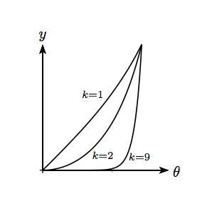
For , we have , so that the curve is close to zero (i.e. much smaller than 1) when is large. This is illustrated in the figure which shows three cases: for the graph is mildly curved; for larger the graph hugs the -axis before taking off. The graphs all pass through the point .
(i) To evaluate the integral, let
| () |
We shall express in terms of using the relation :
To evaluate the second integral, set so that .
Repeating the process gives
The above sum (starting with ) is the same as that in overleaf, so it only remains to evaluate , corresponding to in :
as required.
We deduce the expression overleaf for using the first line of the question. When is very large, is very small, being the area under a graph which is almost zero for almost all of the range of integration. In the limit , we set in which leads immediately to .
(ii) To obtain the formula for , we follow the above method using instead of . This time we have to calculate :
Post-mortem
You might think that the method of obtaining the formula for in this question is rather indirect; one could instead just integrate the formula
| () |
term by term and get the result immediately by setting . The virtue of the method used in the question is that it gives an explicit form (an integral) of the remainder after terms of the series. We were able to show, by means of a sketch, that the remainder tends to zero as tends to infinity; in other words, we showed that the series converges. Although the sketch method of proof is a bit crude, it can easily be made more rigorous once the concept of integration is more carefully defined. On the other hand, integrating () and setting is a bit delicate, since the series only converges for .

