Problem 44:  A differential-difference equation ($✓$ $✓$) 1990 Paper II

A damped system with feedback is modelled by the equation

where $k$ is a given non-zero constant.

Show that (non-zero) solutions for f of the form $\mathrm{f}\left(t\right)=A{\mathrm{e}}^{mt}$, where $A$ and $m$ are constants, are possible provided $m$ satisfies

Show also, by means of a sketch or otherwise, that equation (2) can have 0, 1 or 2 real roots, depending on the value of $k$, and find the set of values of $k$ for which such solutions exist. For what set of values of $k$ do the corresponding solutions of (1) tend to zero as $t\to \infty$?

Comments

Do not be put off by the words at the very beginning of the question, which you do not need to understand. In any case, the question very soon morphs into an investigation of roots of an equation using curve sketching. However, their meaning can be gleaned from the equation itself (sometimes called a differential-difference equation). The left hand side of the equation is the rate of increase of the function $\mathrm{f}$, which may measure the amplitude of some physical disturbance. According to the equation, this is equal to the sum of two terms. One is $-\mathrm{f}\left(t\right)$, which represents damping: this term alone would give exponentially decreasing solutions. The other is a positive term proportional to $\mathrm{f}\left(t-1\right)$: this is called a feedback term, because it depends on the value of $\mathrm{f}$ one year (say) previously. The feedback term could represent some seasonal effect, while the damping term may be caused by some resistance-to-growth factor.

The suggested method of solving the equation is similar to what you might have used for second order linear equations with constant coefficients: you guess a solution (${\mathrm{e}}^{mt}$) and then substitute into the equation to check that this is a possible form of solution and to find the values of $m$ which will work. It is always possible to multiply the exponential by a constant factor, since any constant multiple of a solution is also a solution. (This is a consequence of the linearity of the equation: i.e. no terms involving $\mathrm{f}{\left(t\right)}^2$, $\mathrm{f}{\left(t\right)}^3$, etc.) We can also take linear combinations of solutions to produce a more general solution.

To find the set of values of $k$ which give real solutions of (2), you need to investigate the borderline case, where the two curves $y=m+1$ and $y=k{e}^{-m}$ just touch (and therefore have the same gradient). Remember that the sign of $k$ is not restricted.

Unlike the second order differential equation case, the equation for $m$ is not quadratic; in fact, it is not even polynomial, since it has an exponential term. This means, as we will find, that there may not be exactly 2 solutions; in general, there may be many solutions (e.g. the non-polynomial equation $sinm=0$ has solutions $m=0,\pi ,2\pi ,\dots$) or no solutions (e.g. ${\mathrm{e}}^m=0$ has no solutions). And unlike the differential equation case, we have no idea whether the method is going to work, because there may be solutions of a completely different form. The full analysis of equations such as (1) provides an extraordinarily rich field of study with many surprising results.

Solution to problem 44

We do as we are told to start and substitute $A{e}^{mt}$ into equation (1). After cancelling the overall factor $A$, we get

We can cancel the overall factor ${\mathrm{e}}^{mt}$, but an exponential remains on account of the $\mathrm{f}\left(t-1\right)$ term:

which is equivalent to equation (2) overleaf.

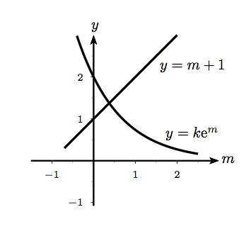
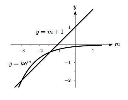
The above sketches show $y=m+1$ and $y=k{\mathrm{e}}^{-m}$ on the same axes, for positive and negative $k$: in the first sketch, $k=2$; in the second $k=-0.1$.

As can be seen from the sketches, equation (2) always has exactly one solution if $k>0$. For $k<0$, there may be two or zero solutions depending on whether the line and curve intersect, or just one solution if they touch. They will touch if there is a value of $m$ such that

the second of these equations being the condition that the gradients (differentiate with respect to $m$ to find the gradient) of the line and curve are the same at the common point. Solving the two equations gives $m=-2$ and $k=-{\mathrm{e}}^{-2}$.

If $0>k>-e^{-2}$, then the curve and line will intersect, so the set of values of $k$ for which equation (2) has solutions is $k>0$ and $-e^{-2}\le k<0$.

The corresponding solutions to equation (1) tend to zero as $t\to \infty$ if and only if $m<0$, because then they are exponentially decreasing rather than increasing.

If $k<0$, we can see from the sketch that the solutions of (2), if there are any (i.e. if $-e^{-2}\le k<0$), occur in the bottom left quadrant, and so $m<0$. The corresponding solutions of (1) will tend to zero.

If $k>0$, the intersection of the graph of $y=k{e}^{-m}$ with the $y$-axis is at $y=k$ whereas the intersection of the graph of $y=m+1$ with the $y$-axis is at $y=1$. For $k\ge 1$, the solution of (2) occurs in the top right quadrant and has $m\ge 0$. For $0<k<1$, the solution occurs in the top left quadrant and has $m<0$.

The range of $k$ for which the solutions tend to zero as $t\to \infty$ is therefore $-e^{-2}\le k<0$ and $0<k<1$.