15. Demographic Sources of
Variation in Fitness

Silke van Daalen and Hal Caswell

© 2024 Silke van Daalen and Hal Caswell, CC BY 4.0 https://doi.org/10.11647/OBP.0251.15

Heritable variation in fitness is required for natural selection, which makes identification of the sources of variation in fitness a crucial question in evolutionary biology. A neglected source of variance is the demography of the population. Demographic processes can generate a large amount of variance in fitness, but these processes are stochastic and the variance results from the random outcomes of survival, development and reproduction, and will therefore be non-heritable. To quantify the variance in fitness due to individual stochasticity, the mean and variance of lifetime reproductive output (LRO) are calculated from age-specific fertility and mortality rates. These rates are incorporated into a stochastic model (a Markov chain with rewards) and the statistical properties of lifetime reproduction — including Crow’s Index of the opportunity for selection — are calculated. We present the basic theory for these calculations, and compare results with empirical measurements of the opportunity for selection. In the case of a historical population in Finland, 57% of the empirically observed opportunity for selection can be explained by individual stochasticity resulting from demographic processes. Analysing the contribution of demography to variance in fitness will improve our understanding of the selective pressures operating on human populations.

Introduction

Natural selection on a trait is an automatic consequence of three conditions: (1) there is variation among individuals, (2) the variation is heritable and (3) the trait is correlated with fitness, so that individuals differing in the trait experience differential reproductive success (Darwin, 1859; Lewontin, 1970; Brandon, 1978; Endler, 1986). Disentangling the underlying sources of variation in fitness, and of traits correlated with fitness, is a critical component of evolutionary biology, because not all variation is heritable or correlated with fitness.

Quantitative genetics provides powerful statistical tools for partitioning phenotypic variance into its components (e.g. Falconer, 1960; Kempthorne, 1957). The total phenotypic variance is customarily partitioned into genetic variance, environmental variance and variance that occurs as a result of gene-environment interactions. The genetic variance is further partitioned into additive and non-additive components (see Figure 1). Additive genetic variance is due to the linear contributions of alleles to the trait, and is the component of variance that determines the response to selection (Falconer, 1960; Lande, 1979). Non-additive variance arises due to dominance effects and epistatic effects. Heritability in the broad sense is the ratio of the genetic variance to the total variance. Heritability in the narrow sense, which determines the response to selection, is the ratio of additive genetic variance to the total variance (Crow and Kimura, 1970, p. 124).

In this chapter, we distinguish demographic analyses from other kinds of population calculations. By the demography of a species, we refer to the life cycle and its stages, the differences among individuals due to those stages, and the stochastic outcomes (surviving or not, reproducing successfully or not) of demographic processes in these stages. The familiar analysis of variance in quantitative genetics was developed with only minimal consideration of demography. As we will show, the contributions of these demographic processes (known as individual stochasticity; see Caswell, 2009) can be sizeable and should not be ignored. Methods now exist to calculate the demographic contributions to variance from standard life table information (Caswell, 2011; van Daalen and Caswell, 2015, 2017) and we will present these methods, together with examples, below.

Fitness and the Response to Selection: Crow’s Index

Selection requires genetic variance, and the rate at which a trait responds to selection depends on the genetic variance in the trait and on the correlation of the trait with fitness. Fitness is, of course, perfectly correlated with itself, and so the response of fitness to selection is a useful starting point for analysis. Crow (1958) derived an index that measures the opportunity for selective improvement in fitness from the variance in fitness.

Suppose that the population contains k trait values and that individuals with trait value i have fitness wi and occur with frequency pi. The mean fitness at a given time is the sum of all possible fitness values weighted by their proportions, w(t) = Σpi wi. The frequency of trait i will change over time according to its current frequency and fitness:

where the mean fitness scales pi(t + 1) so that it sums to one.

Mean fitness in the next generation is w(t + 1) = Σpi (t + 1)wi, which, by replacing pi (t + 1), can be written as

The change in mean fitness from t to t + 1 over time is Δw = w(t + 1) − w(t). Crow (1958) writes this change as a proportion, relative to the mean fitness at time t, to obtain

This is obviously related to Fisher’s fundamental theorem of natural selection, which states that “the rate of increase in fitness of any organism at any time is equal to its genetic variance in fitness at that time” (Fisher, 1930: p. 35).

Crow’s index I gives the proportional rate of increase in fitness when fitness is perfectly heritable, so that all the variance is genetic. The rate of change of any other trait would depend on the correlation of that trait with fitness (Crow, 1958). Crow’s I has been referred to as “the index of total selection”, “the intensity of selection”, and “the opportunity for selection”, the latter of which most accurately represents its interpretation (Crow, 1958; Arnold & Wade, 1984; Cavalli-Sforza & Bodmer, 1999). Crow’s I is an upper limit to the rate of the response to selection, but this limit is realized only if fitness is completely heritable and selection is not frequency-dependent.

Fitness and its Components

The definition and measurement of fitness are matters of great debate in ecology and evolution (e.g. Mills & Beatty, 1979; Metz, Nisbet & Geritz, 1992; Roff, 2008; Barker, 2009). It is clear that fitness is a demographic concept, because it measures the rate at which a particular phenotype or genotype is able to propagate copies of itself to future generations (Fisher, 1930; Dobzhansky, 1951; Hedrick, 1983; Barker, 2009, Metz, Nisbet, and Geritz, 1992). Such a rate is a demographic outcome.

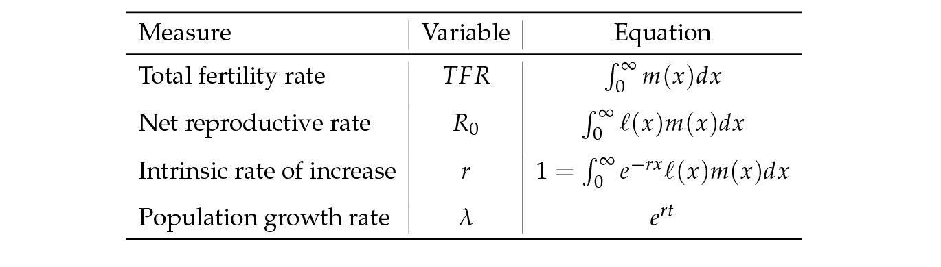
Crow’s definition of fitness avoids this; it simply states that the number of individuals with trait i increases by a factor ωi in each generation, without specifying how that factor is determined. Fisher (1930) suggested the use of the intrinsic rate of increase r (the Malthusian parameter in Fisher’s terminology) as a measure of fitness. It is calculated from survival and fertility schedules as shown in Table 1 (Fisher, 1930; Charlesworth, 1994). Metz and others have made a case for taking a similar, but more stringent measure of fitness: the rate of increase of a rare mutant in a resident population in a given environment, as measured by the dominant Lyapunov exponent (Metz, Nisbet, and Geritz, 1992; Metz, 2008). The discrete-time version of the population growth rate is λ = ert.

All these demographic measures incorporate the life cycle, the changes that happen to individuals as they develop through the life cycle and some measure of rate of increase. Most evolutionary studies, however, must be satisfied with components of fitness that capture some aspects of survival, reproduction, growth, etc. even if they do not suffice to compute λ. The component perhaps most closely related to λ is lifetime reproductive output (LRO). The mean LRO, if measured as the number of daughters per female, is equivalent to the net reproductive rate R₀ (see Table 1), which is the per-generation rate of increase and, as such, serves as an indicator of population growth, decline or stability (Heesterbeek, 2002; Caswell, 2001). Both R₀ and LRO are often taken as a proxy for fitness (Grafen, 1988; Clutton-Brock, 1988; Newton, 1989; Partridge, 1989; Stearns, 1992; Roff, 1992; Charlesworth, 1994).

Lifetime reproductive output is, however, a demographic consequence of the complete set of stage-specific vital rates throughout the life cycle. It integrates the rates of survival, development and reproduction across age classes or stages, no matter how those stages are connected. Thus, LRO can be calculated from life tables or projection matrices, provided that they contain information on age-specific mortality and fertility (Caswell, 2001; 2011).

Table 1: Mathematical definitions of a few familiar fitness measures.

Individual Stochasticity in LRO

Demography is a source of variance in fitness. In general, variance among individuals arises from two sources. One is heterogeneity: genuine differences among individuals, which translate into differences in the rates of mortality and fertility experienced by those individuals at any age or stage. This is the variance that is decomposed into the familiar environmental and genetic components (Figure 1). The other source is individual stochasticity, variance that arises from the stochastic outcomes of probabilistic transitions (living or dying, giving birth or not, maturing or not, etc.) within the life cycle. Variance due to individual stochasticity is unavoidable in any quantity that results from demography, but it is invisible in fitness calculations that ignore the demographic structure of the population.

Consider an extreme example, where every individual experiences the age-independent mortality rate µ. The longevity of individuals has an exponential distribution with a mean of 1/µ (life expectancy), and a variance of 1/µ². This variance is a result of individual stochasticity, because by assumption we have eliminated every source of heterogeneity from this example.

The same principle holds when the vital rates depend on age — conditional on age, individuals experience the same rates and probabilities, but may differ in their outcomes. Calculating the amount of variance in LRO produced by stochastic events in the life cycle has been a long-standing problem, which has recently been solved (Caswell, 2011; van Daalen, and Caswell, 2017). In the next section we will present these results, and we will apply them to Finnish population data as an example.

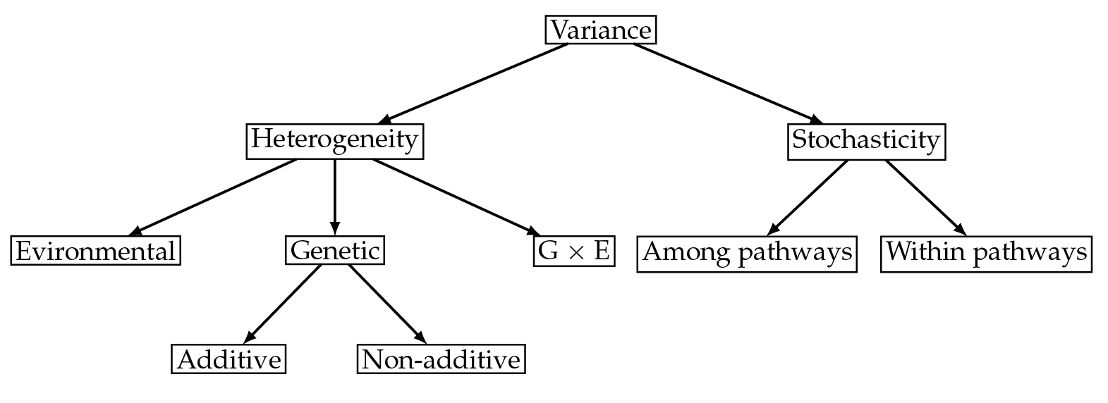
Fig. 1 Variance among individuals is caused by heterogeneity, i.e. actual differences between individuals, and by stochasticity, i.e. differences in outcome by chance.

A Markov Chain Model for Stochasticity in LRO

Individual stochasticity can be calculated by incorporating demographic processes into a stochastic model for individuals. An individual in age class i may survive and advance to the next age class (with probability p_i) or die (with probability 1 − p_i). It will reproduce with probability f_i.1 The probabilistic nature of surviving or dying at a given age class causes random variation among the pathways individuals follow through their life course. Similar random variation is caused within pathways by probabilistic fertility (Figure 1).

These probabilities are captured in a stochastic model framework referred to as absorbing Markov chains with rewards (Caswell, 2011; Caswell and Kluge, 2015; van Daalen and Caswell, 2015; 2017). The Markov chain describes the movement of individuals among a set of states, in this case, among age classes. An individual of any age has a probability of surviving to the next age class. These probabilities appear on the sub-diagonal of the transition matrix of the Markov chain (see Box I). Individuals who die are captured into the absorbing state of death. This model keeps track of all possible trajectories that individuals take through their life course, from birth to eventual death, and the probabilities of each.

At each step in its trajectory, an individual may accumulate offspring. These offspring are treated as “reward” in the Markov chain model. Rewards accumulate until the individual dies. Thus, defining rewards as offspring in this analysis leads directly to a measure of lifetime reproductive output. The statistical moments of rewards are incorporated into a set of reward matrices (see Box II). For humans, we assume that the fertility at age i is the probability of producing a single child, which implies the higher moments of the reward matrix follow a Bernoulli distribution. With this structure, a Markov chain with rewards model incorporates the full range of stochasticity, as it arises partly as a consequence of probabilistic survival and transitions, and partly as a consequence of probabilistic success at reproduction.

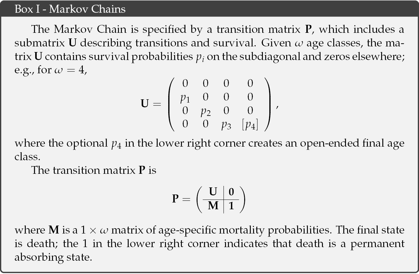
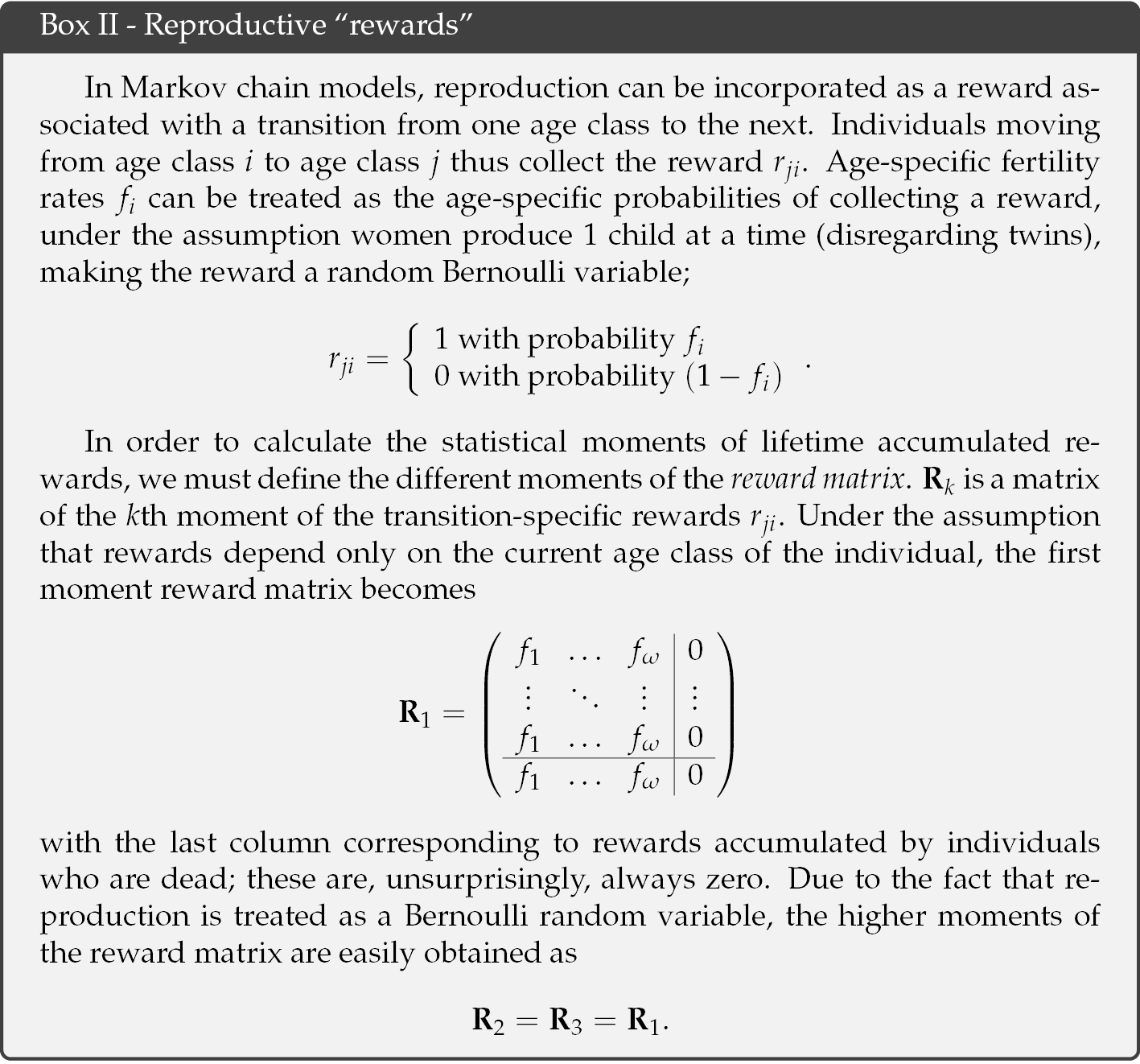
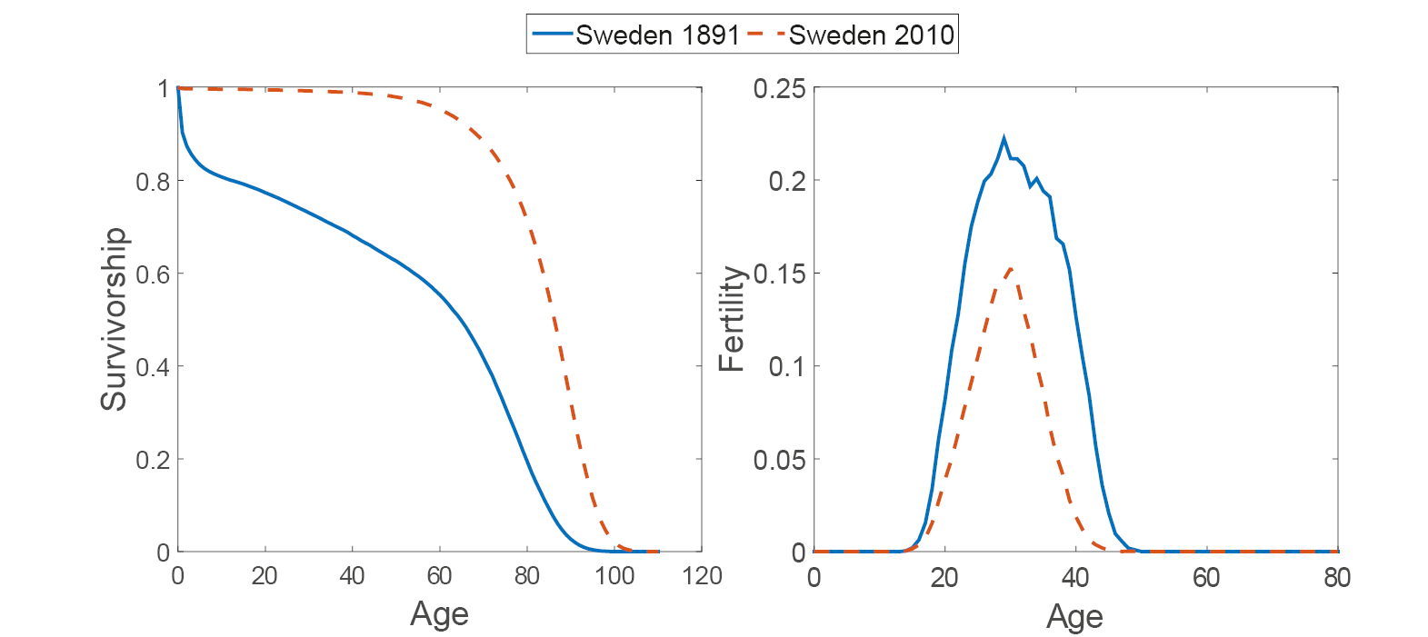
Fig. 2 Survivorship (left panel) and fertility (right panel) for Sweden at two different points in time, 1891 (solid blue line) and 2010 (dashed red line).

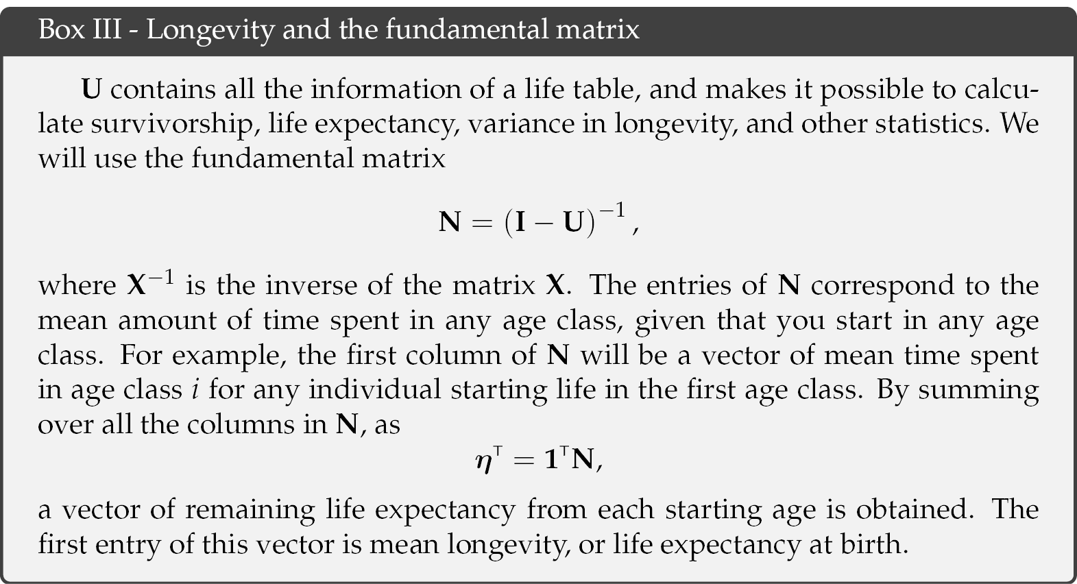
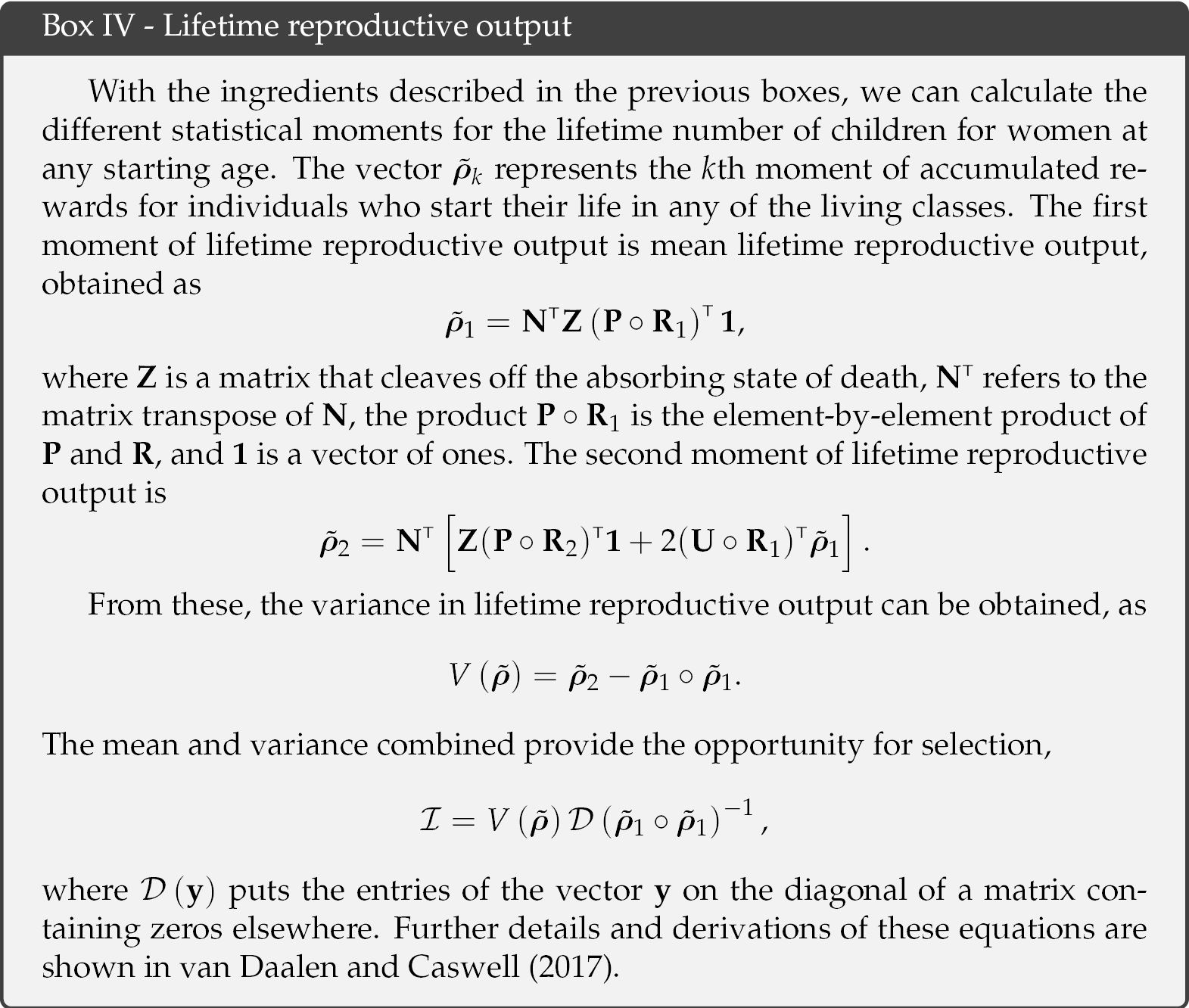
The accumulated number of children over the lifetime of an individual, i.e. lifetime reproductive output, is then a function of the Markov chain P, the reward matrix R_i, and the fundamental matrix N. The latter is obtained from the Markov chain and provides information on the occupation times of different age classes and longevity (see Box III). Calculating Crow’s index of the opportunity for selection requires the first two moments of LRO (see Box IV), but calculation of all higher moments is also possible (van Daalen and Caswell, 2017).

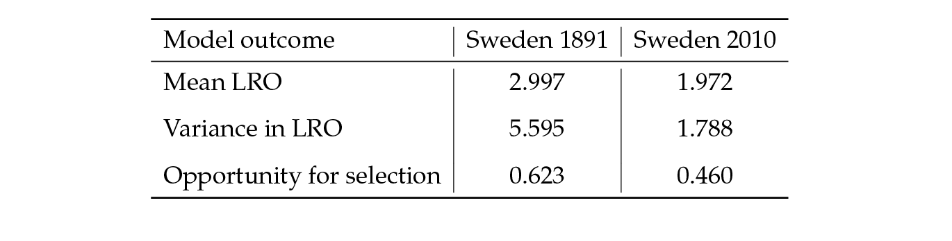
As an example, consider Sweden in 1891 and 2010 (Figure 2). Survival was higher in 2010 than in 1891; fertility was lower in 2010 than in 1891. The Markov chain with rewards calculation shows that, given these rates, a Swedish woman in 1891 would produce an average of three children (of either sex) over her lifetime. The variance in lifetime reproduction, among a cohort of women identically experiencing the rates of 1891, would be 5.6. Crow’s index would be I = 0.62. This variance is due to the random outcomes of the age-specific probabilities of survival and reproduction. By 2010, mean LRO had declined to two children. The variance, again among individuals identically experiencing 2010 rates, would be 1.8, with Crow’s I = 0.46 (see Table 2).

Table 2: Mean lifetime reproductive output, variance and opportunity for selection calculated using Markov chains with rewards for Sweden at two points in time. The model was parameterized using mortality and fertility as shown in Boxes I and II.

It is important to be clear about what this variance reflects. The calculations assume that every woman experiences the same fertility and mortality rates at every age, so there is no heterogeneity involved on which to select. This lack of heterogeneity, genetic or otherwise, means that this estimate of Crow’s I is based on demographic variation with a completely non-heritable basis. We therefore refer to it as an apparent, rather than a real opportunity for selection.

These values of Crow’s I due to individual stochasticity are not unusual. In an analysis of fertility during the second demographic transition, we calculated Crow’s index for a set of forty developed countries (van Daalen and Caswell, 2015), based on age-specific demographic data from the Human Mortality Database (Human Mortality Database, 2014), the Human Fertility Database (Human Fertility Database, 2014) and the Human Fertility Collection (Human Fertility Collection, 2014). We found values of Crow’s I in the range of roughly 0.25 to 1.0, increasing slightly between 1960 and 2000, with a slight decrease after 2000 (see Figure 3). Van Daalen and Caswell (2017) found values in a similar range for two hunter-gatherer populations and the high-fertility Hutterites.

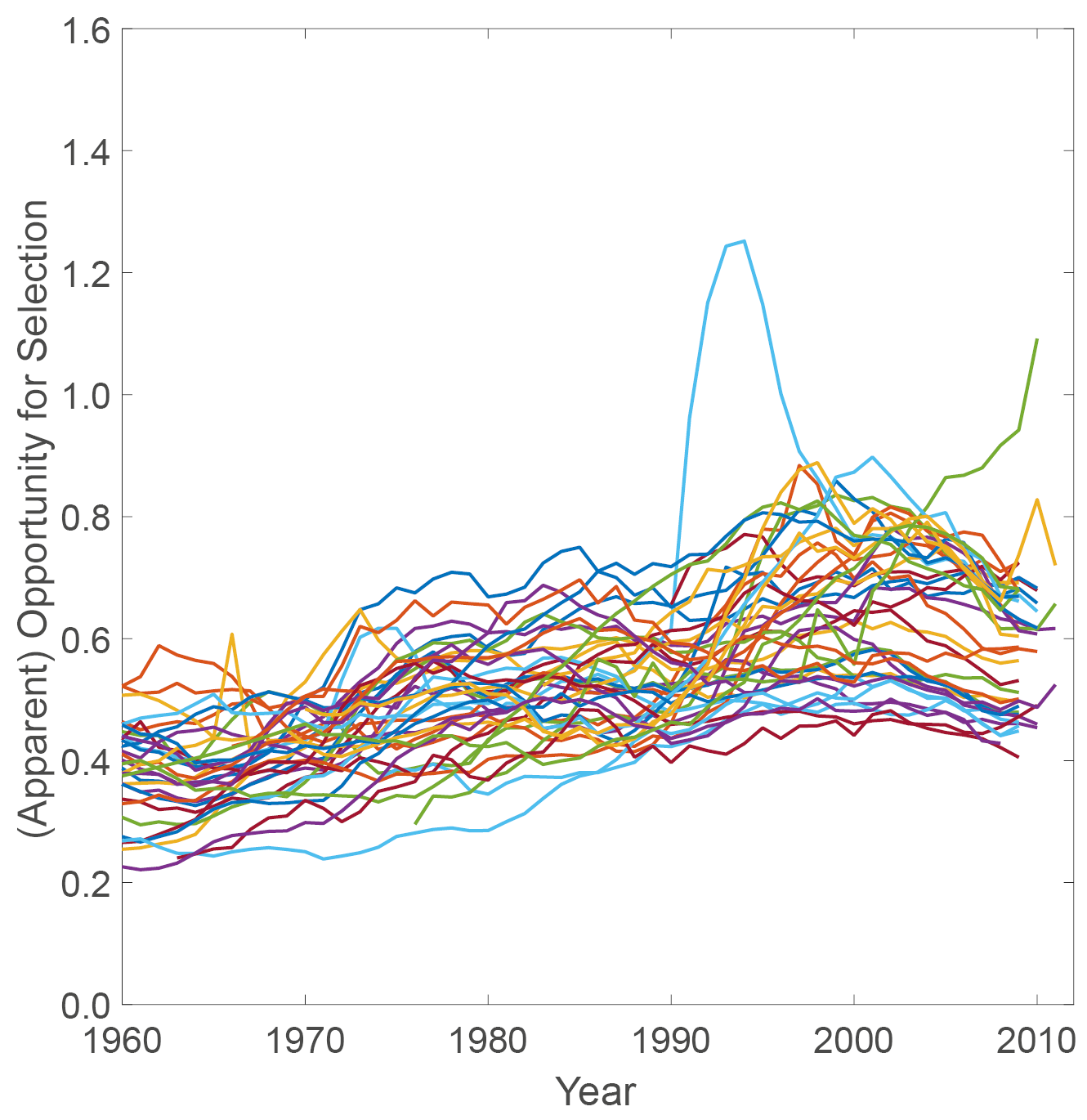
Fig. 3 Apparent opportunity for selection calculated using the Markov chain with rewards method for forty developed countries between 1960 and 2010. Values fall broadly within a range of 0.2–0.8.

Empirical Estimates of the Opportunity for Selection in Human Populations

Given individual lifetime data, it is possible to make empirical estimates of Crow’s I. Such data have been used to investigate reproduction in a number of human populations. The index is often partitioned by sex (Crow, 1962; Wade, 1979; Brown, Laland and Borgerhoff Mulder, 2009), by episodes of selection (Crow, 1958; Arnold and Wade, 1984) or by the type of selection. The latter partitioning was developed by Wade (1979; 1995), who derived an expression for the opportunity for sexual selection from Bateman’s observations on variance in number of mates (Bateman, 1948).

Table 3: Empirical measures of opportunity for selection (OFS) in reproductive success of women in 18 populations, with a median of 0.34, and an interquartile range of 0.16–0.46.

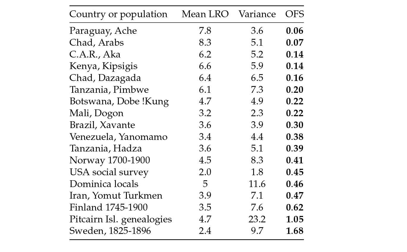
Brown, Laland and Borgerhoff Mulder (2009) have compiled such empirical estimates of the sex-specific opportunity for selection in eighteen human populations. In Table 3 we have tabulated their estimates as female opportunity for selection. The values (median=0.34, interquartile range=0.16–0.46) are similar to those produced by individual stochasticity in typical human life tables, with only three populations exceeding 0.5. The estimates of opportunity for selection were higher in males in most populations, something that might reflect sex roles, but for which there was not sufficient evidence (Brown, Laland and Borgerhoff Mulder, 2009).

Brown, Laland, and Borgerhoff Mulder (2009) also found differences among mating systems (i.e. monogamy, serial monogamy, polygyny, etc.) in the degree to which male opportunity for selection outweighed female opportunity for selection. A more robust study by Moorad et al. (2011) showed that a shift in the mating system of a frontier population in Utah between 1830 and 1894 reduced the opportunity for selection over time. The opportunity for selection was high in males in 1830 (approximately 1.1) and decreased by almost half around mid-century, corresponding to the shift from polygyny to monogamy. For women, the opportunity for selection was quite stable across this time period (around 0.5–0.6).

Nulliparity as an Issue

A confounding issue in empirical measurements of variance in LRO is the treatment of individuals that do not reproduce at all (nulliparous individuals), either because they die before reproducing or simply never produce children. These individuals are often excluded from estimates, thereby underestimating the variance in lifetime reproduction. The study by Moorad et al. (2011) is an apparent exception, but to our knowledge, the only study of opportunity for selection in human populations that includes explicit counts of nulliparous individuals is that of Courtiol et al. (2012). They used detailed church records of preindustrial populations in Finland between 1760 and 1849 to obtain counts of lifetime reproductive output for all women, nulliparous or not.

Courtiol et al. (2012) estimate the opportunity for selection for women as I = 2.03, which is distinctly higher than other empirical estimates (Table 3) and higher than estimates calculated from life tables (Figure 3). They found no evidence for effects of social status on the opportunity for selection. The opportunity for selection was again higher in males, estimated at around 2.52. The larger values in this study are most likely due to the inclusion of nulliparous individuals in the estimates of Crow’s I, and as such they are a benchmark estimate, at least for a preindustrial European population.

Pre-industrial Finland: Variance and Stochasticity

The empirical estimate of the opportunity for selection reported by Courtiol et al. (2012) for Finnish women in the late eighteenth to mid-nineteenth century provides a valuable opportunity for comparison with the level of variance due to individual stochasticity that is implied by the mortality and fertility schedules of that era. To make such a comparison, we require mortality and fertility schedules as comparable as possible to those of the Finnish population represented by the parish register data. If the variance in LRO due to individual stochasticity is similar to the observed value, invoking heterogeneity to explain the variance is, strictly speaking, not necessary without additional evidence (Steiner and Tuljapurkar, 2012).

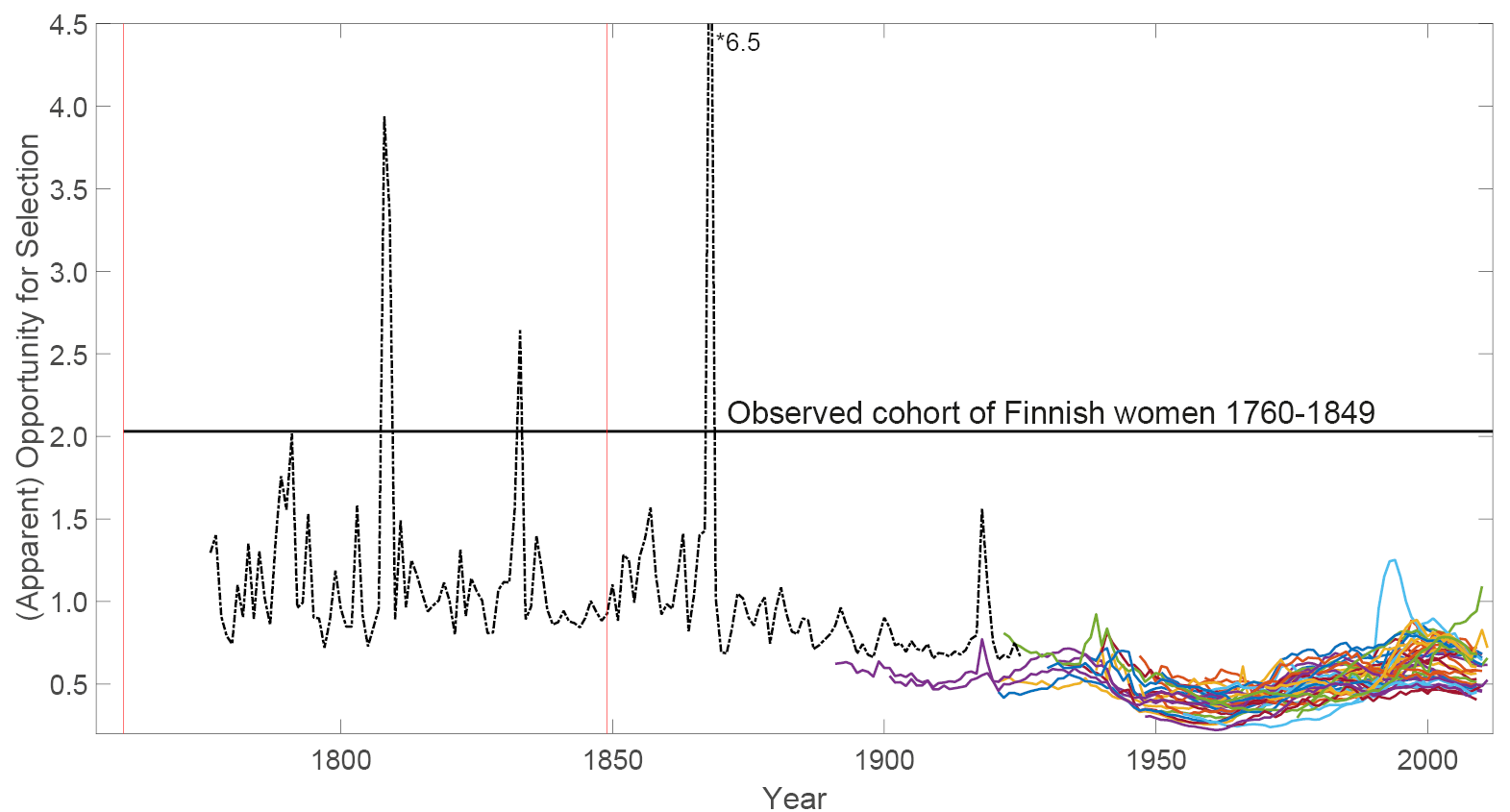
Fig. 4 The straight back line represents the empirically measured opportunity for selection for Finnish women living between 1760 and 1849; the window of time wherein this measure was obtained is indicated by vertical red lines. The black dash-dotted line represents apparent opportunity for selection obtained from life table data on Finnish women living between 1776 and 1925. Peaks correspond to famines and wars, times when mortality was higher. The apparent opportunities for selection for forty developed countries are shown as a reference in the bottom-right corner of the figure (coloured lines).

Turpeinen (1979) reported estimates of age-specific mortality and fertility for Finland, from 1776 to 1925. We interpolated Turpeinen’s results from five-year age classes (or, for the first years of life, two-year age classes) to single-year age classes using cubic splines. We used the resulting mortality schedules to create the matrix U, and the fertility data to create the reward moment matrices R₁ and R₂, for each year (see Boxes I and II), and calculated the resulting values of Crow’s I, as shown in Figure 4.

The mean value of opportunity for selection between 1776 and 1849 was 1.15, which is 2–3 times the value for current developed countries. This value declined gradually from the mid-nineteenth century to the typical modern values. This is at least partly a result of the reduction in mortality since that time, because such changes reduce I (see the sensitivity analysis results in van Daalen and Caswell, 2017).

Like all empirical estimates, the values of Crow’s I reported by Courtiol et al. (2012) reflect both sources of variance in LRO (see Figure 1). Compared to their value of 2.03, the value of apparent opportunity for selection implies that slightly more than half of Crow’s I can be accounted for by individual stochasticity. The remainder, approximately 0.8, could be due to heterogeneity. This heterogeneity could be genetic, or it could be non-genetic, such as marital status, parity or geographical location (Figure 1).

Discussion

Natural selection is, at heart, a demographic process, concerned as it is with the differential propagation of genes, genotypes or traits (Metcalf and Pavard, 2007). This demographic basis is recognized in the calculation of fitness (measured as some rate of increase that integrates survival and reproduction) and fitness components (measured by indices that capture some, but not all, aspects of survival and reproduction).

To this familiar concept, we must also add demography as a source of variance in fitness and its components, due to individual stochasticity. The existence of random events within the life cycle makes this stochasticity an unavoidable result, implicit in any demographic model. It has now been shown, by a variety of methods, that individual stochasticity creates significant amounts of variance in human and non-human populations (e.g. Caswell, 2009; Tuljapurkar, Steiner and Orzack, 2009; Steiner, Tuljapurkar and Orzack, 2010; Caswell, 2011; Steiner and Tuljapurkar, 2012; van Daalen and Caswell, 2015; Hartemink, Missov and Caswell, 2017; van Daalen and Caswell, 2017).

Human life tables imply a degree of individual stochasticity in LRO that is sufficient to create values of Crow’s I that are on the same order as empirical measurements of variance in lifetime reproduction. This result has several implications. It provides a baseline against which empirical measurements can be compared. It serves as a neutral model (sensu Steiner and Tuljapurkar, 2012), eliminating all sources of heterogeneity, and implies the need to search for evidence of heterogeneity in order to invoke it as a source of the variance. The variance produced by individual stochasticity can be expected to reduce the efficacy of natural selection, by masking variance produced by genetic differences (Steiner and Tuljapurkar, 2012).

The methods presented here (and in more detail in Caswell, 2011; van Daalen and Caswell, 2017) make it possible to calculate the individual stochasticity in lifetime reproductive output implied by any set of mortality and fertility schedules. This opens the way for increasingly detailed study of the demographic contribution to variance in fitness, and its implications for human evolutionary demography.

Acknowledgements

References2

Arnold, S. J., and M. J. Wade. 1984. ‘On the Measurement of Natural and Sexual Selection: Theory’, Evolution, 38.4: pp. 709–19, https://doi.org/10.1111/j.1558-5646.1984.tb00344.x

Barker, J. S. F. 2009. ‘Defining Fitness in Natural and Domesticated Populations’, in Adaptation and Fitness in Animal Populations, ed. Julius van der Werf and others (Dordrecht: Springer), pp. 3–14, https://doi.org/10.1007/978-1-4020-9005-9_1

Bateman, A. J. 1948. ‘Heredity – Abstract of Article: Intra-Sexual Selection in Drosophila’, Heredity, 2: pp. 349–68. https://doi.org/10.1038/hdy.1948.21

Brandon, R. N. 1978. ‘Adaptation and Evolutionary Theory’, Studies in History and Philosophy of Science Part A, 9.3: pp. 181–206. https://doi.org/10.1016/0039-3681(78)90005-5

Brown, G. R., K. N. Laland, and M. Borgerhoff Mulder. 2009. ‘Bateman’s Principles and Human Sex Roles’, Trends in Ecology & Evolution, 24.6: pp. 297–304, https://doi.org/10.1016/j.tree.2009.02.005

Caswell, H. 2014. ‘A Matrix Approach to the Statistics of Longevity in Heterogeneous Frailty Models’, Demographic Research, 31: pp. 553–92, https://doi.org/10.4054/DemRes.2014.31.19

—. 2011. ‘Beyond R₀: Demographic Models for Variability of Lifetime Reproductive Output’, PLoS ONE, 6: pp. 1–21, https://doi.org/10.1371/journal.pone.0020809

—. 2001. Matrix Population Models: Construction, Analysis, and Interpretation, 2nd edn (Sunderland: Sinauer Associates).

—. 2009. ‘Stage, Age and Individual Stochasticity in Demography’, Oikos, 118.12: pp. 1763–82, https://doi.org/10.1111/j.1600-0706.2009.17620.x

Caswell, H., and F. A. Kluge, ‘Demography and the Statistics of Lifetime Economic Transfers under Individual Stochasticity’, Demographic Research, 32: pp. 563–88, https://doi.org/10.4054/DemRes.2015.32.19

Cavalli-Sforza, L. L., and W. F. Bodmer. 1999. The Genetics of Human Populations (North Chelmsford: Courier Corporation).

Charlesworth, B. 1994. Evolution in Age-Structured Populations (Cambridge: Cambridge University Press).

Clutton-Brock, T. H. 1988. Reproductive Success (Chicago: University of Chicago Press).

Courtiol, A., J. E. Pettay, M. Jokela, A. Rotkirch, and V. Lummaa, 2012. ‘Natural and Sexual Selection in a Monogamous Historical Human Population’, Proceedings of the National Academy of Sciences, 109.21: pp. 8044–49, https://doi.org/10.1073/pnas.1118174109

Crow, J. F. 1962. ‘Population Genetics: Selection’, in Methodology in Human Genetics, ed. by W. J. Burdette (San Francisco: Holden-Day).

—. 1958. ‘Some Possibilities for Measuring Selection Intensities in Man’, Human Biology, 30.1: pp. 1–13. https://www.jstor.org/stable/41449168

Crow, J. F., and M. Kimura. 1970. An Introduction to Population Genetics Theory (New York: Harper and Row).

van Daalen, S. F., and H. Caswell. 2015. ‘Lifetime Reproduction and the Second Demographic Transition: Stochasticity and Individual Variation’, Demographic Research, 33: pp. 561–88, https://doi.org/10.4054/DemRes.2015.33.20

—. 2017. ‘Lifetime Reproductive Output: Individual Stochasticity, Variance, and Sensitivity Analysis’, Theoretical Ecology, 10: pp. 1–20, https://doi.org/10.1007/s12080-017-0335-2

Darwin, C. 1859. On the Origin of Species by Means of Natural Selection, or the Preservation of Favoured Races in the Struggle for Life (London: John Murray).

Dobzhansky, T. G. 1951. Genetics and the Origin of Species (New York: Columbia University Press).

Endler, John A. 1986. Natural Selection in the Wild (Princeton: Princeton University Press).

Falconer, D. S. 1960. Introduction to Quantitative Genetics (New York: Ronald Press Company). http://archive.org/details/introductiontoq00falc

Fisher, R. A. 1999. The Genetical Theory of Natural Selection: A Complete Variorum Edition (Oxford: Oxford University Press).

Grafen, A. 1988. ‘On the Uses of Data on Lifetime Reproductive Success’, in Reproductive Success, ed. by T. H. Clutton-Brock (Chicago: University of Chicago Press), pp. 454–71.

Hartemink, N., and H. Caswell. 2018. ‘Variance in Animal Longevity: Contributions of Heterogeneity and Stochasticity’, Population Ecology, 60.1–2: pp. 89–99, https://doi.org/10.1007/s10144-018-0616-7.

Hartemink, N., T. I. Missov, and H. Caswell. 2017. ‘Stochasticity, Heterogeneity, and Variance in Longevity in Human Populations’, Theoretical Population Biology, 114: pp. 107–16, https://doi.org/10.1016/j.tpb.2017.01.001

Heesterbeek, J. A. 2002. ‘A Brief History of R _o and a Recipe for its Calculation’, Acta Biotheoretica, 50: pp. 189–204, https://doi.org/10.1023/A:1016599411804

‘Human Fertility Collection’, 2014. Human Fertility Collection. Max Planck Institute for Demographic Research (Germany) and Vienna Institute of Demography (Austria). www.fertilitydata.org

‘Human Fertility Database’, 2014. Human Fertility Database. Max Planck Institute for Demographic Research (Germany) and Vienna Institute of Demography (Austria). http://www.humanfertility.org

‘Human Mortality Database’, Human Mortality Database. University of California, Berkeley (USA), and Max Planck Institute for Demographic Research (Germany). www.mortality.org

Jenouvrier, S., L. M. Aubry, C. Barbraud, H. Weimerskirch, and H. Caswell. 2017. ‘Interacting Effects of Unobserved Heterogeneity and Individual Stochasticity in the Life History of the Southern Fulmar’, Journal of Animal Ecology, 87.1: pp. 212–22, https://doi.org/10.1111/1365-2656.12752

Kempthorne, O. 1957. An Introduction to Genetic Statistics (New York: John Wiley & Sons, Inc.).

Klug, H., K. Lindström, and H. Kokko. 2010. ‘Who to Include in Measures of Sexual Selection Is No Trivial Matter’, Ecology Letters, 13.9: pp. 1094–1102, https://doi.org/10.1111/j.1461-0248.2010.01495.x

Lande, R. 1979. ‘Quantitative Genetic Analysis of Multivariate Evolution, Applied to Brain: Body Size Allometry’, Evolution, 33.1: pp. 402–16, https://doi.org/10.2307/2407630

Lewontin, R. C. 1970. ‘The Units of Selection’, Annual Review of Ecology and Systematics, 1.1: pp. 1–18. https://doi.org/10.1146/annurev.es.01.110170.000245

Metcalf, C. J. E., and S. Pavard. 2007. ‘Why Evolutionary Biologists Should Be Demographers’, Trends in Ecology & Evolution, 22.4: pp. 205–12, https://doi.org/10.1016/j.tree.2006.12.001

Metz, J. A. J. 2008. ‘Fitness’, in Encyclopedia of Ecology, ed. by Sven E. Jørgensen and Brian D. Fath (Oxford: Academic Press), pp. 1599–1612, https://doi.org/10.1016/B978-008045405-4.00792-8

Metz, J. A. J., R. M. Nisbet, and S. A. H. Geritz. 1992. ‘How Should We Define “Fitness” for General Ecological Scenarios?’, Trends in Ecology & Evolution, 7.6: pp. 198–202, https://doi.org/10.1016/0169-5347(92)90073-K

Mills, S. K., and J. H. Beatty. 1979. ‘The Propensity Interpretation of Fitness’, Philosophy of Science, 46.2: pp. 263–86, https://doi.org/10.1086/288865

Moorad, J. A., D. E. L. Promislow, K. R. Smith, and M. J. Wade. 2011. ‘Mating System Change Reduces the Strength of Sexual Selection in an American Frontier Population of the 19th Century’, Evolution and Human Behavior, 32.2: pp. 147–55, https://doi.org/10.1016/j.evolhumbehav.2010.10.004

Newton, I. 1989. Lifetime Reproduction in Birds (New York: Academic Press).

Partridge, L. 1989. ‘Lifetime Reproductive Success and Life History Evolution’, in Lifetime Reproduction in Birds, ed. by I. Newton (New York: Academic Press), pp. 421–40.

Roff, D. A. 2008. ‘Defining Fitness in Evolutionary Models’, Journal of Genetics, 87.4: pp. 339–48, https://doi.org/10.1007/s12041-008-0056-9

—. 1993. Evolution Of Life Histories: Theory and Analysis (New York: Chapman and Hall).

Stearns, S. C. 1992. The Evolution of Life Histories (Oxford: Oxford University Press).

Steiner, U. K., and S. Tuljapurkar. 2012. ‘Neutral Theory for Life Histories and Individual Variability in Fitness Components’, PNAS, 109.12: pp. 4684–89, https://doi.org/10.1073/pnas.1018096109

Steiner, U. K., S. Tuljapurkar, and S. H. Orzack. 2010. ‘Dynamic Heterogeneity and Life History Variability in the Kittiwake’, Journal of Animal Ecology, 79.2: pp. 436–44, https://doi.org/10.1111/j.1365-2656.2009.01653.x

Tuljapurkar, S., U. K. Steiner, and S. H. Orzack. 2009. ‘Dynamic Heterogeneity in Life Histories’, Ecology Letters, 12.1: pp. 93–106, https://doi.org/10.1111/j.1461-0248.2008.01262.x

Turpeinen, O. 1979. ‘Fertility and Mortality in Finland since 1750’, Population Studies, 33.1: pp. 101–14, https://doi.org/10.1080/00324728.1979.10412779

Wade, M. J. 1979. ‘Sexual Selection and Variance in Reproductive Success’, The American Naturalist, 114.5: pp. 742–47, https://doi.org/10.1086/283520

—. 1995. ‘The Ecology of Sexual Selection: Mean Crowding of Females and Resource-Defence Polygyny’, Evolutionary Ecology, 9.1: pp. 118–24, https://doi.org/10.1007/BF01237701