4. Presenting Conclusions from Assessed Evidence

William J. Sutherland^1,2, Tatsuya Amano^3,4, Nicolas Boenisch⁵, Samantha H. Cheng^6,7, Alec P. Christie^1,2,8, H. Charles J. Godfray⁹, Matthew J. Grainger¹⁰, Angela R. McLean⁹, William H. Morgan¹, Nancy Ockendon¹¹, Nicola P. Randall¹², Ullrika Sahlin¹³, Thomas B. White¹

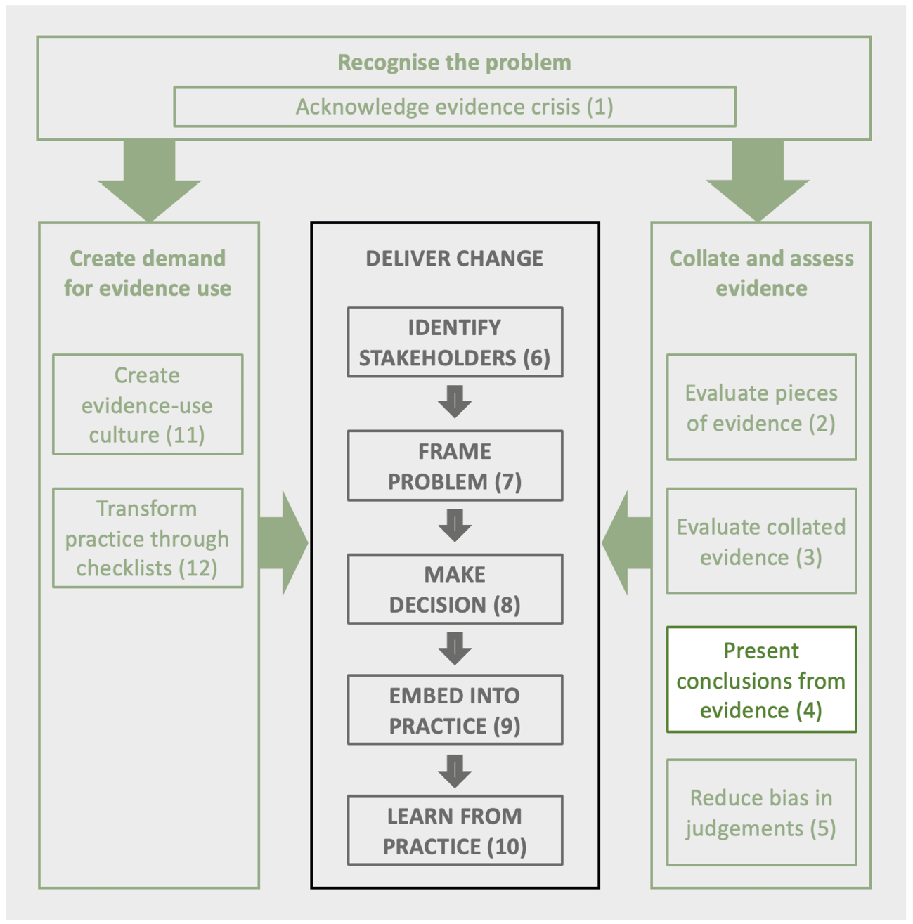
Applying evidence builds on the conclusions of the assessment of the evidence. The aim of the chapter is to describe a range of ways of summarising and visualising different types of evidence so that it can be used in various decision-making processes. Evidence can also be presented as part of evidence capture sheets, argument maps, mind maps, theories of change, Bayesian networks or evidence restatements.

¹ Conservation Science Group, Department of Zoology, University of Cambridge, The David Attenborough Building, Pembroke Street, Cambridge, UK.

² Biosecurity Research Initiative at St Catharine’s College (BioRISC), St Catharine’s College, Cambridge, UK.

³ School of Biological Sciences, University of Queensland, Brisbane, 4072 Queensland, Australia

⁴ Centre for Biodiversity and Conservation Science, The University of Queensland, Brisbane, 4072 Queensland, Australia

⁵ Foundations of Success Europe, 7211 AA Eefde, The Netherlands

⁶ Center for Biodiversity and Conservation, American Museum of Natural History, New York, NY 10026, USA

⁷ Global Science, World Wildlife Fund, Washington, D.C., USA

⁸ Downing College, Regent Street, Cambridge, UK

⁹ Oxford Martin School, University of Oxford, Oxford, UK

^1o Norwegian Institute for Nature Research (NINA), PO Box 5685 Torgarden, 7485 Trondheim, Norway

¹¹ Endangered Landscapes Programme, Cambridge Conservation Initiative, David Attenborough Building, Pembroke Street, Cambridge, UK

¹² Centre for Evidence-based Agriculture, Harper Adams University, Newport, Shropshire, UK

¹³ Centre for Environmental and Climate Science, Lund University, Lund, Sweden

What does the evidence say? This is a common question and one that is critical to the process of decision-making (Chapter 8) and applying evidence, whether writing plans or deciding upon policies (Chapter 9). The aim of this chapter is to present a range of means of presenting evidence that gives a fair summary whilst making clear any limitations or biases.

This chapter considers the general principles, reviews the various elements that are involved in finding and presenting evidence, describes some of the main types of evidence and how these might be presented, and describes some approaches for presenting multiple pieces of evidence.

4.1 Principles for Presenting Evidence

In applying evidence, it is important to understand the conclusions drawn and the likelihood that those conclusions are accurate and relevant. The core general principles for presenting evidence (see Box 4.1) are designed to reduce the risk that the evidence is misapplied due to the conclusions being presented incorrectly; the limitations not being made clear; or because the conditions are very different.

In practice, evidence is presented in a range of formats that differ in the detail provided. In some cases, such as reports and assessments, the key evidence is likely to be well documented with details of the source and assessment of quality. However, in practice, much evidence is provided by experts. In this case, the responsibility is on the expert to ensure that if caveats are needed then they are provided (for example, ‘although the evidence is weak it seems…’, ‘the evidence is conflicting but my interpretation is…’, ‘the only studies are on lizards but it seems likely that snakes would respond the same way’). Thus if a responsible evidence-based expert provides no caveat then it should be reasonable to assume the expert holds no such concerns. In practice, it is worth checking if the expert does this and also checking the details for key assumptions.

4.2 Describing Evidence Searches

Understanding how the evidence is presented is key for interpreting the results, as it indicates how complete the evidence is, and the likelihood of any bias.

4.2.1 Describing the types and results of searching

Here, we describe how different types of evidence could be obtained. Table 4.1 outlines possible content for describing a range of search methods.

Table 4.1 Suggested possible content, with examples, for presenting different means of searching for evidence.

4.2.2 Constraints on generality statements

Evidence collations often provide general conclusions, for example, to cover wide geographic areas or groups of species. However, these are based on the evidence available, which often has taxonomic, habitat and geographic biases (Christie et al., 2020a, 2020b). For example, an action may have been assessed as being beneficial for birds, but all of the studies testing the action may have been carried out in one habitat type for a small number of species. Therefore, before making any decisions it is vital to consider the evidence in more detail to assess its relevance for your study species or system and to state the relevance and any constraints in any outcome, for example, there are numerous good studies showing this resulted in higher breeding success, but all the studies are on Salmonids.

4.3 Presenting Different Types of Evidence

The aim of this section is to consider how different types of evidence, including describing costs, may be summarised.

4.3.1 Conservation Evidence summaries

Conservation Evidence collates and summarises individual studies on a topic in a consistent manner to ease comparisons and ensure all the key components are included. For example:

A search of Conservation Evidence for ‘tree harvesting’ found seven individual studies and seven relevant actions.

Conservation Evidence uses a standard format for describing studies that test interventions, which may be of wider use. The following colour-coded format is here illustrated with an example.

A [TYPE OF STUDY] in [YEARS X-Y] in [HOW MANY SITES] in/of [HABITAT] in [REGION and COUNTRY] [REFERENCE] found that [INTERVENTION] [SUMMARY OF ALL KEY RESULTS] for [SPECIES/HABITAT TYPE]. [DETAILS OF KEY RESULTS, INCLUDING DATA]. In addition, [EXTRA RESULTS, IMPLEMENTATION OPTIONS, CONFLICTING RESULTS]. The [DETAILS OF EXPERIMENTAL DESIGN, INTERVENTION METHODS and KEY DETAILS OF SITE CONTEXT]. Data was collected in [DETAILS OF SAMPLING METHODS].

For the type of study there is a specific set of terms that are used (Table 4.2). For the results, for the sake of brevity, only key results relevant to the effects of the intervention are included. For Site context only those nuances that are essential to the interpretation of the results are included.

As an example:

A replicated, randomized, controlled, before-and-after study in 1993–1999 of five harvested hardwood forests in Virginia, USA (1) found that harvesting trees in groups did not result in higher salamander abundances than clearcutting. Abundance was similar between treatments (group cut: 3; clearcut: 1/30 m2). Abundance was significantly lower compared to unharvested plots (6/30 m2). Species composition differed before and three years after harvest. There were five sites with 2 ha plots with each treatment: group harvesting (2–3 small area group harvests with selective harvesting between), clearcutting and an unharvested control. Salamanders were monitored on 9–15 transects (2 x 15 m)/plot at night in April–October. One or two years of pre-harvest and 1–4 years of post-harvest data were collected.

(1) Knapp S.M., Haas C.A., Harpole D.N. and Kirkpatrick, R.L. 2003. Initial effects of clearcutting and alternative silvicultural practices on terrestrial salamander abundance. Conservation Biology 17: 752–62.

Table 4.2 The terms used to describe study designs in Conservation Evidence summaries.

* Note that ‘controlled’ is mutually exclusive from ‘site comparison’. A comparison cannot be both controlled and a site comparison. However, one study might contain both controlled and site comparison aspects e.g. study of fertilised grassland, compared to unfertilised plots (controlled) and natural, target grassland (site comparison).

4.3.2 Systematic maps

Systematic maps (Section 3.2.1) are overviews of the distribution and nature of the evidence found in literature searches. Standardised descriptive data from individual studies are usually extracted and presented within searchable databases or spreadsheets, which accompany written systematic reports and the descriptive statistics. As critical appraisal of included studies does not usually take place in systematic maps, to avoid vote-counting, systematic maps authors do not usually summarise the outcomes of included studies.

Their description includes statistics about the studies included, such as the number of papers on different sub-topics or from different regions, a summary of the quantity and the quality of the evidence identifying areas of strong evidence and knowledge gaps. It also includes a description of the process used (including whether Collaboration for Environmental Evidence guidelines and ROSES reporting standards are adopted), date carried out, and sources and languages searched. For example:

Adams et al. (2021) mapped out the literature on the effects of artificial light on bird movement and distribution and found 490 relevant papers. The most frequent subjects were transportation (126 studies) and urban/suburban/rural developments (123) but few were from mineral mining or waste management sectors. Many studies are concerned with reducing mortality (169 studies) or deterring birds (88). The review followed a published protocol and adopted the Collaboration for Environmental Evidence guidelines and ROSES reporting standards. The search, on August 21 2019, was for literature in English in the Web of Science Core Collection, the Web of Science Zoological Record, Google Scholar and nine databases.

Or for a brief version:

One good quality, recent systematic map of the English literature (Adams et al., 2021) found 88 papers on using light to deter birds.

4.3.3 Systematic reviews

Systematic reviews use repeatable analytical methods to extract secondary data and analyse it and can also be carried out for qualitative studies. Their description includes the objective, number of studies, statistics and the main results. Description of any meta-analysis should describe the summary or averaged effect size (e.g. the mean difference between having the focal intervention and not having it), the uncertainty around this (e.g. 95% confidence limits) and the heterogeneity (variability in reported effect sizes) between studies included in the analysis and the main results of any meta-regression used to explore the drivers of the between-study heterogeneity. A description of the process used (whether Collaboration for Environmental Evidence guidelines and ROSES reporting standards are adopted), date carried out and sources and languages searched, should also be described.

For example, for the systematic review given in Chapter 3:

An English language systematic review, following Collaboration for Environmental Evidence guidelines, produced 78 primary studies that assess whether tree retention at harvest helps to mitigate negative impacts on biodiversity, (Fedrowitz et al., 2014). Meta-analysis showed that overall species richness (15 studies) and abundance (50 studies) were significantly (hedges d p<0.001) higher with tree retention at harvest compared to clear cutting. However, there were significant differences among taxonomic groups in richness-response to retention cuts compared with un-harvested forests.

Or more briefly:

A good quality meta-analysis of 78 studies showed tree harvest resulted in more biodiversity than clear cutting, but the responses varied between groups.

4.3.4 Dynamic syntheses

Metadataset (see Section 3.7) provides a means for running meta-analysis for the subject of concern. For example for invasive species the user can select the species, countries included action and outcome. It generates a Forest plot with effect sizes and confidence intervals, a paragraph summarising the main conclusions and a funnel plot showing the precision of studies against their effect size results as one check for publication bias. Their description includes the comparison selected and geography included, the response ratio, statistical significance, the number of studies and papers and any significant heterogeneity.

For example, the example shown in Figure 3.4, of analysing the effectiveness of different action on invasive Japanese knotweed could be summarised as follows.

The effect of chemical and mechanical control on the abundance of invasive Japanese knotweed (Fallopia japonica) was selected for analysis. Chemical control reduced abundance by 63% lower compared to the untreated control (response ratio = 0.37; significance P = 0.0084; 193 data points from 13 studies in 12 publications). For physical disturbance, the abundance was 16% lower than the control but this was not statistically significant (response ratio = 0.84; P = 0.579; 27 data points from 8 studies in 8 publications). For both analyses, there was significant heterogeneity between data points (P < 0.0001).

Or for a brief version

Analysis using metadataset showed a significant 63% reduction in Japanese knotweed abundance when treated with herbicide but a non-significant 16% reduction with physical disturbance.

4.3.5 Conservation Evidence actions

State date, name of action, assessment category and describe the nature of the evidence in relation to the topic of interest. One key principle is to be careful of ‘vote counting’ — presenting the number of studies showing different results when these might differ in quality.

The action ‘Add mixed vegetation to peatland surface’ (2018 synopsis) has 18 studies and is classified as Beneficial. Seventeen replicated studies looked at the impact on Sphagnum moss cover (five were also randomised, paired, controlled, before-and-after): in all studies Sphagnum moss was present (cover ranged from <1 to 73%), after 1–6 growing seasons, in at least some plots. Six of the studies were controlled and found that Sphagnum cover was higher in plots sown with vegetation including Sphagnum than in unsown plots. Five studies reported that Sphagnum cover was very low (<1%) unless plots were mulched after spreading fragments.

Or for a brief version:

The 17 replicated studies on Conservation Evidence looking at adding mixed vegetation showed in all cases there was some Sphagnum in at least some plots but in five cases at low density.

4.3.6 Costs of actions

Most conclusions will wish to give some indication of cost, yet, as described in Chapter 2, the reporting of costs is usually unsatisfactory. Either costs are not given or are given without stating what is included. One solution is the standardised collation and reporting of costs to help think through and report the direct costs of conservation actions. Iacona et al. (2018) developed a framework to help record the direct accounting costs of interventions. These steps are outlined below. Major accounting costs include the costs of consumables, capital expenditure, labour costs and overheads.

• Step 1: State the objective and outcome of the intervention.
• Step 2: Provide context, and the method used for the intervention.
• Step 3: When, where and at what scale was the intervention implemented?
• Step 4: What categories of cost are included? (see Table 2.4) What are these costs and how might they vary with context?
• Step 5: State the currency and date for the reported costs.

White et al. (2022b) created a further 6-step framework for thinking through the wider economic costs and benefits of different conservation actions that can be used to assess cost-effectiveness:

• Step 1: Define the intervention/programme.
• Step 2: Outline the costing perspective and reporting level.
• Step 3: Define the alternative scenario.
• Step 3: Define the types of cost and benefits included or excluded (see Table 2.4).
• Step 5: Identify values for the included cost categories.
• Step 6: Record cost metadata (e.g. date, currency).

In a similar style to the layout of the CE effectiveness summary paragraphs (Section 4.3.2) the following suggestions give suggested standard frameworks for reporting different elements of costs in line with cost reporting frameworks (e.g. Iacona et al. 2018). This is a flexible format covering a range of levels of detail.

For marginal intervention costs for the conservation organisation (probably the majority of the reported costs):

First sentence on total costs and what is included:

Total cost was reported as XX in [currency; ] in [year] ([XX USD]) at [information on the scale e.g. XXkm, per hectare; breakdown not provided]. Costs are given over a [XX] time horizon and a discount rate of [XXX] applied. They included [types of cost] and excluded [types of cost] /

Possible additional sentence on the financial benefits of action.

Financial benefit was reported as: XX in [currency; [XX equivalent USD]; breakdown not provided), resulting in a net cost of XX. The benefits only included [types of benefit].

Additional sentence on the breakdown of the specific costs if provided.

Cost breakdown: XX [XX USD] for XX materials, XX [XX USD} for XX hours/days of labour, XX [XX USD] for overheads, XX [XX USD] for capital expenditure… [continue for all types of cost reported] (For further details see original paper).

For project level or organization costs, where the costs of interventions are given as part of a broader package:

Total cost of the action was reported as part of a [describe type and scale of conservation project]. The cost of this project was reported as XX in [currency; no breakdown provided] including [specific activities]. Costs are given over a [XX] time horizon and a discount rate of [XXX] applied. They included [types of cost] and excluded [types of cost]

Note: Where costs or benefits are incurred by actors other than the conservationist/researcher, this should be noted. E.g., ‘the total included …. Opportunity costs to local communities, payments made by volunteers to travel to the nature reserve.’

As examples:

Total costs reported as £1,000 GBP in 2022 ($1,200 USD) for 2km of fencing. Costs are given over a 5 year time horizon with no discount rate applied. Cost breakdown: £100/2km for wire fencing and £900 for 5 day of labour for 4 staff. Financial benefit was reported as £200 ($240 USD), resulting in a net cost of £800 ($960 USD). Benefits included the reduced loss of livestock to local stakeholders.

Total cost reported as €10,000 EUR in 2008 ($12,000 USD) for the translocation of 10 animals (£1000 / animal). Cost breakdown: €2000 [$2400 USD] for tracking devices, supplementary food, and veterinary supplies, €6000 [$7200 USD} for one staff employed by the project for two months and €2000 [$2400 USD] for overheads (project management). Financial benefits reported as €10,000 ($12,000 USD), resulting in a net cost of €0 ($0 USD). Benefits included the estimated tourism value of each reintroduced eagle, although benefits are accrued by the wider sector.

As an example of a brief version:

In 2008, this project cost an extra US$550 comprising $250 for fuel and $300 for chainsaw and safety equipment.

4.4 Presenting Evidence Quality

4.4.1 Information, source, relevance (ISR) scores

Figure 4.1 shows a range of information, source, reliability (ISR) cuboids as introduced in Chapter 2. For a particular assumption in a particular context, the ISR score is an assessment of whether a particular piece of evidence, whether a systematic review or observation, is relevant, and was generated in a reliable manner and from a source considered reliable. Such assessments will often not be public, especially if it would be embarrassing for the source to discover how their reliability is assessed. In other cases, it may be possible to compare different examples of the same type of evidence using predefined criteria or tools available for specific evidence types. One such tool is the CEESAT checklist, https://environmentalevidence.org/ceeder/about-ceesat/, which enables users to appraise and compare the reliability of the methods and/or reporting of evidence reviews and evidence overviews (such as systematic maps) by assessing the rigour of the methods used in the review, the transparency of the reporting, and the limitations of the review or overview.

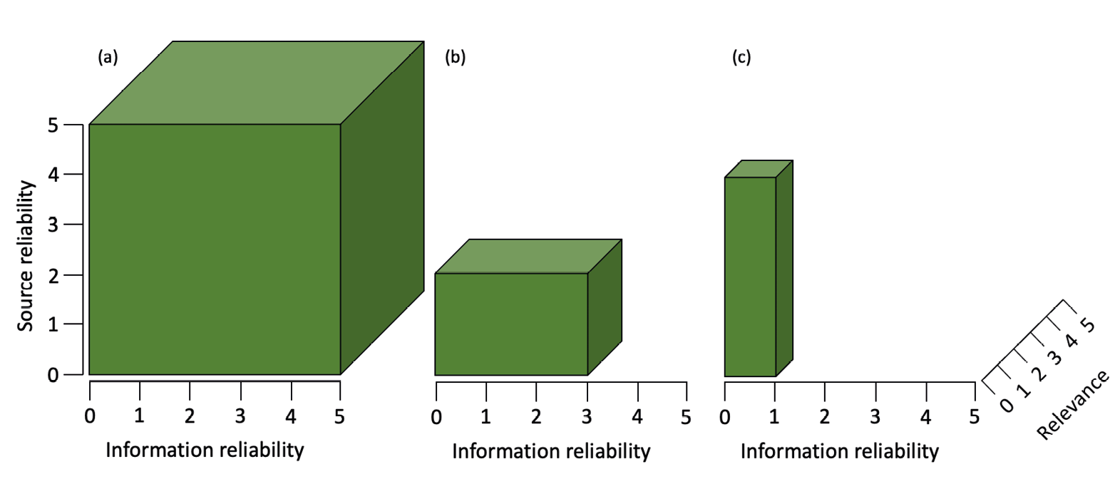
Figure 4.1 Cuboids of different strengths of evidence can range in weight from 0 (no weight) to 125 (5³). In practice they will usually be cuboids of different dimensions. (a) strongly supported on all three axes; ISR = 5.5.5, (b) limited information and source reliability but highly relevant; ISR = 3,2,2 (c) high source but little information reliability or relevance; ISR = 1,1,5. (Source: authors)

Chapter 2 outlines some factors that influence the scores given for each of the three ISR elements. Our suggestion is that ISR becomes a standard way of assessing the weight of different pieces of evidence including different types of knowledge with the ISR score at the end of the claim: During lockdown, when the reserve was closed, cranes were said to have nested within 3m of the trackway in part of a reserve where they have never nested before (I = 3, S = 4, R = 5).

The weight of a piece of evidence can then be presented by multiplying the three ISR axes up to a maximum weight of 125 (5³). Of course, if the value of one axis is zero, meaning that an element of the evidence either cannot be trusted or is judged to be irrelevant, then the weight is zero. Table 4.3 suggests how these weights can be converted into descriptions of the strength of evidence for a single piece of evidence.

Table 4.3 Conversion of weights of single pieces of evidence (from multiplying three axes) into descriptions of evidence strengths.

4.5 Balancing Evidence of Varying Strength

Whilst in some cases, evidence will either clearly refute or support an assumption (as in the above examples), in many situations there is a range of relevant evidence that varies in its strength and direction in relation to a particular assumption. This is often the case when assessing the effectiveness, costs, acceptability, or feasibility of actions, where evidence can, for example, show an action to be beneficial to different extents, have no effect, or have negative impacts. Where this is the case, one approach, modified from Salafsky et al. (2019), is to imagine placing the various pieces of evidence along a balance according to the direction and magnitude of the effect they report, from large negative effects, through to large positive effects (in this case, effectiveness; Christie et al., 2022) (Figure 4.2).

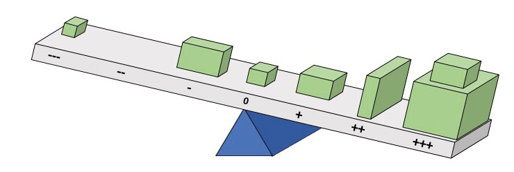
Figure 4.2 A means of visualising the balance of evidence behind an assumption. The pieces of evidence are placed on the balance according to the extent to which it supports or rejects the assumption. The greater the tilt the greater the confidence in accepting (or rejecting) an assumption. (Source: authors)

How can this visualisation be converted into a conclusion? Table 4.4 provides a way of assessing the evidence for an assumption about an action. The cumulative evidence score is the sum of the weights of each block of evidence. The weight of each block can be calculated by multiplying the ISR (information, source, relevance) scores (Section 4.2.2). Adding the weights of all evidence blocks together gives the cumulative weight of evidence. The mean effectiveness category comes from assessing the effectiveness associated with each piece of evidence and then taken as the average (the weighted median — place the evidence in order of effectiveness, add up the ISR values until you reach the figure that is half the value for the cumulative evidence, take the effectiveness linked to piece of evidence).

Table 4.4 Converting the combined evidence into statements of the strength of evidence. The maximum score for a piece of evidence is 125 (5 x 5 x 5) so strong evidence requires, say, one really strong study conducted in a manner that minimises bias and overwhelming evidence requires over two high-quality studies.

4.5.1 Statements of effectiveness

The cumulative evidence and mean effectiveness can be combined to give statements of the effectiveness for actions — the Strategic Evidence Assessment (SEA) model (Table 4.5). These statements can then be used in other processes, such as writing management plans or funding applications.

Table 4.5 The Strategic Evidence Assessment model. Converting the combined evidence into statements of effectiveness combining the scores from Table 4.4 with effectiveness.

4.5.2 Words of estimative probability

When President Kennedy was deciding whether to proceed with the proposal for the disastrous Bay of Pigs invasion of Cuba, the US Joint Chiefs of Staff stated that the proposal had a ‘fair chance’ of success, which Kennedy interpreted as likely to work. The Chiefs actually meant that they judged the chances of success as ‘3 to 1 against’ (Wyden 1980). As a result of such lessons, the accepted least ambiguous approach is to attempt estimating probabilities. Studies have shown, at least in medicine, that giving natural frequencies ‘Three out of every 10 patients have a side effect from this drug’ leads to fewer problems of interpretation than probabilities, such as ‘You have a 30% chance of a side effect from this drug’ (Gigerenzer and Edwards, 2003).

Some dislike judging probabilities (how certain we are about something) or estimating frequencies (how often something happens), partly because it seems to give unjustified accuracy. An alternative approach is to express likelihoods in the form of standardised terms. Table 4.6 gives the language for communicating probabilities recommended by the Intergovernmental Panel on Climate Change (IPCC, 2005). Table 4.7 gives the opposite: examples of some ‘weasel’ words that are likely to be ambiguous and so should be avoided.

Table 4.6 Terms suggested by the IPCC (2005) for referring to probabilities.

Table 4.7 Examples of ‘weasel’ terms likely to be ambiguous.

4.6 Visualising the Balance of Evidence

In some cases it may be particularly informative to visualise the collated evidence base, ideally communicating both the weight of the evidence pieces and the results they found. Here we present two different options for visualising a collated evidence base that are best suited to slightly different types of results.

4.6.1 Ziggurat plots

Ziggurat plots (Figure 4.3) are best suited to results where the outcomes can be expressed categorically (e.g. varying discrete levels of effectiveness). The width of each bar represents its ISR score (out of 125) with studies piled in order of ISR score to give a ziggurat shape. This has the merit of showing the distribution of the evidence.

In some cases, the median may be a poor representation of the distribution, for example, because the results are strongly bimodal. In this case add a comment e.g. ‘median effect size mixed, but results strongly bimodal’.

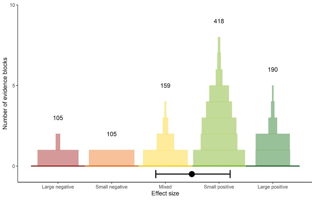
Figure 4.3 A ziggurat plot in which each study is a horizontal bar whose width is the information reliability, source reliability, and relevance (ISR) score (up to 125). The studies are collated for different categories of effectiveness. The number above each pile of evidence blocks shows the total evidence score for that pile. In order to derive an average effect size, we defined effect size categories as consecutive integers (large negative = -2; small negative = -1; mixed = 0; small positive = 1; large positive = 2) and calculated the weighted mean (filled black point) and 95% confidence intervals. The confidence interval was calculated by bootstrapping the weighted mean. (Source: authors). The following R code can be used to carry out this process, which we have adapted from code produced by Stackoverflow users Tony D and Ben https://stackoverflow.com/questions/46231261/bootstrap-weighted-mean-in-r. Text in quote marks must be altered by the user:

library(boot)

df <- data.frame(x= “degree of support”, w= “ISR score”)

wm <- function(d,i){

  return(weighted.mean(d[i, 1], d[i, 2]))

}

bootwm <- boot(df, wm, R=10000)

boot.ci(boot.out = bootwm)

Figure 4.4 shows a range of possible outcomes. In some cases, the evidence may be clear and convincingly show either a positive effect or no effect. In others the results may be bimodal, for example, if combining studies of reptiles but lizards and snakes show very different responses. In other cases, the responses may be unclear — perhaps as a range of different unknown variables are important.

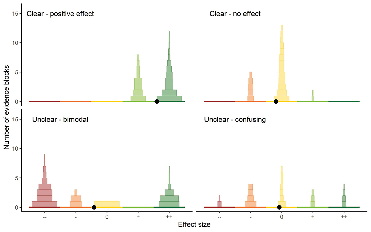
Figure 4.4 A range of possible outcomes of ziggurat plots. Those on the top show clear results, with either a moderately large effect size (left) or evidence for negligible effect (right). Those underneath show unclear effects as either bimodal (left) or scattered results (right). The filled black point shows the average effect size, calculated as the weighted mean. (Source: authors)

4.6.2 Weighted histogram plots

For continuous results (an effect size, or counts of a particular species, for example) however, a ziggurat plot may hide useful information, and the collated evidence base can be better visualised with a weighted histogram plot (Figure 4.5). Sources of evidence are ordered by the magnitude of the result they report, and the height of the bar is the IRS score (out of 125). Evidence pieces that report the same effect sizes are stacked on top of each other.

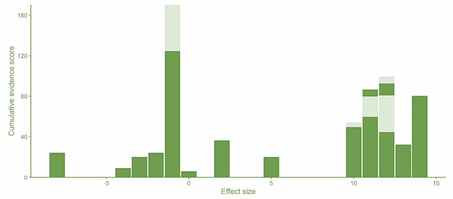
Figure 4.5 A weighted histogram plot in which each piece of evidence is represented by a vertical bar, whose height is the information reliability, source reliability, and relevance (ISR) score. Evidence pieces are arranged in order of the magnitude of the effect size, and where they report the same effect size, they are stacked on top of each other, with alternating colours for each evidence piece in the stack. (Source: authors)

4.7 Synthesising Multiple Evidence Sources

Combining knowledge sources is key. The evidence that decision makers draw on will usually be a combination of scientific knowledge, local knowledge and experience. For example, when managing a reserve, much of the decision making will be based on the experience and local knowledge of the reserve manager and team (‘I think this area is too close to the forest for the species to breed’, for example), informed by knowledge from the local community, local naturalists, fishers, etc and scientific knowledge that has generality.

4.7.1 Evidence review summary statements

The result of the collation or analysis can also be presented in a summary. The aim is to describe the results so that they provide a summary of the amount and nature of the evidence (e.g. quality/reliability, coverage: species, habitats, locations), what it tells us (e.g. effects on key outcome metrics), and any limitations. The different elements of this chapter can be combined, as shown in Table 4.8, to provide a summary of the evidence.

Table 4.8 The different main elements of summarising evidence described in this chapter with an illustrative sentence.

Such summaries can highlight knowledge clusters and thus gaps in the evidence, which are important to take into consideration. However, it is important that summaries are not used to vote count, i.e. draw conclusions based on the number of studies showing positive vs negative results, which is usually a misleading method of synthesis (Stewart and Ward, 2019). Studies are generally not directly comparable or of equal value, and factors such as study size, study design, reported metrics, and relevance of the study to your situation need to be taken into consideration, rather than simply counting the number of studies that support a particular interpretation. Chapter 2 provides suggestions for describing single studies.

In the UK three replicated randomised controlled experiments showed that adding a collar and bell to domesticated cats reduced the predation rate of small mammals by about a half; one of these also showed that effects were similar for bells and a collar-mounted sonic device. Experiments outside the UK showed that a pounce protector (a neoprene flap that hangs from the collar) stopped 45% of cats from catching mammals altogether. A study in the USA showed cats provided with brightly patterned collars brought home fewer mammals than did cats with no collars in autumn, but not in spring. In all cases the cats had a history of bringing back whole prey and the catches were recorded by their owners.

Or for a brief version:

Domesticated cats took roughly half as many small mammals if fitted with collar and bell, collar and sonar device or a neoprene flap hanging from the collar. Brightly coloured collars were less effective.

4.7.2 Evidence capture sheets

Perhaps the most straightforward method for bringing together multiple sources of evidence is to use an evidence capture sheet. Table 4.9 presents an example of such a sheet, with each row constituting a different source of evidence, and each column providing vital information about the validity of the source and the result that it presents. While evidence capture sheets comprehensively communicate the key information of each source of evidence, they stop short of providing an overall conclusion of what the evidence base says.

Table 4.9 Example of tabular presentation of evidence for a proposed project that plans to introduce natural grazing with ponies to the montado habitat in Iberia to increase biodiversity. I = information reliability, S = source reliability, R = relevance all on 0–5 scales. Note the evidence strength is for the particular problem rather than an overall assessment.

a. E.g. peer-reviewed article, expert opinion, grey literature report, personal experience.

b. E.g. synthesis, experimental, observational, anecdotal, theoretical/modelling.

c. Was the result strongly positive, weakly positive, mixed, or no effect?

d. How convincing is the evidence? Depends on the type of evidence, for example, may depend on experimental design and sample size. (0–5)

e. Is the source biased or independent? (0–5)

f. Does it apply to your problem? This will depend on habitat, geography or socio-economic similarity. (0–5)

4.7.3 Argument maps

Argument maps, also called argument diagrams, have three main roles: easing the creation of a logical argument, presenting the basis of an argument so it is easy to follow and reframing an existing argument so making the assumptions, logic and any gaps transparent. The heart of the argument map is to present the case for and against a position in a logical manner. Their merit is that, if done well, they organise and clarify the evidence and reasoning for a contention. These can be done collectively as a way of understanding the basis of any disagreement. They have the considerable advantage that they can easily be converted into text for a decision maker to make the final decision. If using a software package this conversion can be done automatically.

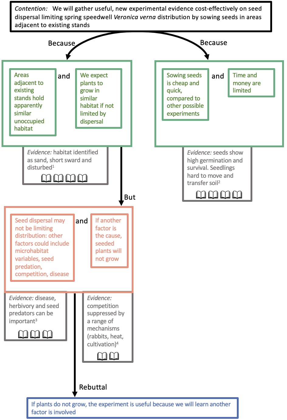
Figure 4.6 An example of an argument map to decide whether or not to introduce a plant to new locations. The main elements are: main contention, premise, counterargument, rebuttal and evidence.  = overwhelming evidence;  = strong evidence;  = moderate evidence;  = weak evidence;  = negligible evidence. The evidence is elaborated in Box 4.2. (Source: authors)

They start with a statement, the main contention, that could be correct or not. The arguments for it being right, the premises, are then listed followed by the arguments for it being wrong, the counterarguments. Co-premises are two statements that both have to be correct. Lines are only drawn between boxes to specify that something is a reason to believe or a reason not to believe something else. The process forces the logic as to whether you should believe the claim and why or why not.

There are three basic rules (https://www.reasoninglab.com/wp-content/uploads/2013/10/Argument-Maps-the-Rules.pdf):

1. The Rabbit Rule (you cannot pull a rabbit out of the hat by magic): every significant word, phrase or concept appearing in the contention must also appear in one of the premises; i.e. every term appearing above the line has to appear below the line. In the example here the terms are sow, spring speedwell, seeds, adjacent areas, distribution, and dispersal.
2. The Holding Hands Rule: every term appearing below the line has to appear above; if something appears in a premise but not in the contention, it must appear in another premise.
3. The Golden Rule: every simple argument has at least two co-premises.

Figure 4.6 shows an argument map created by members of the Breckland Flora Group (Jo Jones, David Dives, Julia Masson, Tim Pankhurst, Norman Sills, William Sutherland, and James Symonds) guided by Mark Burgman. They are interested in planning a reintroduction programme for spring speedwell Veronica verna. Creating this map helped think through the logic for carrying out an experiment to assess whether the species is restricted in range due to lack of dispersal or whether there it is constrained by very specific, but not fully understood, habitat requirements.

Argument maps can easily be sketched out, but there are numerous argument-mapping tools available. Argument mapping has been adopted by the New Zealand government for biosecurity analyses.

4.7.4 Mind maps

Mind maps, as popularised by Buzan (1974), express the relationships between different aspects of a problem. They are also sometimes called spider diagrams or brainstorms. Although often considered as a means of note taking, they can also be used for generating new ideas. Of relevance here they can be used to summarise information around an issue. They are a less structured process than a theory of change or argument map and so are useful for pulling together information to provide a clear account of the components of the issue. One advantage of summarising with such a visual model is that it makes the logic explicit and thus invites further comments. They can be drawn by hand or created using various packages available. These then can be created by a person or team putting together the strands of evidence.

These are created by starting with a central idea or topic, placed in the middle of the map. Branches are then added to this central topic. Each branch is then explored. If the evidence is extracted it can be assessed and added. Another option is to draw a preliminary map based on expert opinion and then adjust as evidence is added.

Figure 4.7 shows an example of a mind map created after a group discussion with experts (Malcolm Ausden, Jennifer Gill, Rhys Green, Jennifer Smart, William Sutherland, and Des Thompson). Box 4.3 lists some supporting evidence. This is intended to be illustrative of the process rather than a comprehensive review of the literature and concepts.

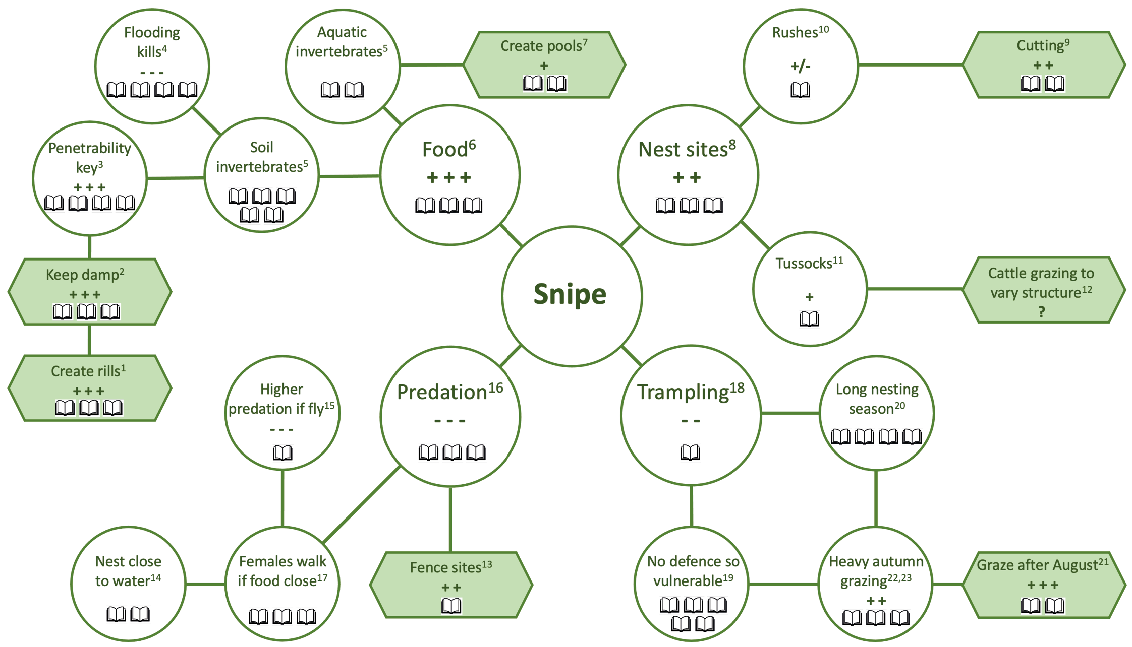
Figure 4.7 A mind map of possible means of managing lowland grassland habitat to improve the common snipe Gallinago gallinago population.  = overwhelming evidence;  = strong evidence;  = moderate evidence;  = weak evidence;  = negligible evidence; ? = no evidence; - - - = considerable harm; - - = moderate harm; - = minor harm; 0 = no effect; +/- = mixed effect; + = little benefit; ++ = moderate benefit; +++ = considerable benefit. See Box 4.3 for the evidence sources. (Source: authors)

In practice most decisions appear to comprise an exploration of components of the issue, rather like an informal mental version of a mind map, followed by a pronouncement of the conclusion. Our experience is that it is often unclear what is justifying the decision. A sketched version of the discussion provides a reminder of the issues and helps force consideration of the components.

4.7.5 Evidence underlying theories of change

A theory of change (CMP, 2020) is a series of causally linked assumptions about how a team thinks its actions lead to intermediate results and to target outcomes (see Chapter 7 for further details). Displaying a theory of change in a strategy pathway diagram (see an example in Figure 4.8 below, repeated from 7.3) facilitates the identification of analytical questions and assumptions that can be tested with evidence.

Once evidence is collected, theories of change can provide the backbone to assess the evidence and contextualise it for a respective conservation action. Often, evidence capture sheets (Table 4.10) are used to relate available evidence to the theory of change and form the basis for drawing overall conclusions about key questions and assumptions, and the effectiveness of the strategy pathway.

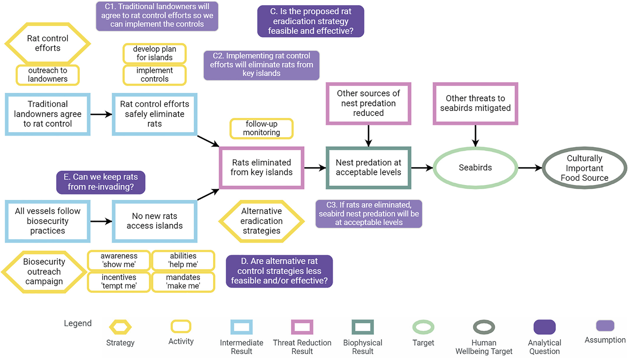
Figure 4.8 A theory of change pathway showing analytical questions and assumptions. This example is derived from several different real-world rat eradication projects. Note, assumptions for questions D and E are not shown. (Source: Salafsky et al., 2022, CC-BY-4.0)

Table 4.10 Summary of current evidence for analytical questions relating to the theory of change shown in Figure 4.7. (Source: Salafsky et al., 2022)

4.7.6 Bayesian networks

Bayesian networks (BNs), as outlined in Box 4.4, are powerful statistical models that represent suspected, theorised or known causal relationships between variables supported by data and knowledge (i.e. evidence) (Jensen, 2001; Stewart et al., 2014). They comprise a network of nodes (i.e. variables or factors) connected by directed arcs (i.e. edges, links or arrows) contextualising the underlying probabilistic relationships. BNs can be built by combining a range of data sources including empirical evidence and expert elicitation. These models are particularly useful because they explicitly and mathematically incorporate uncertainty in a transparent way (Landuyt et al., 2013). Due to the graphical nature of BNs, complex information can be represented in an intuitive manner that is easily interpreted by non-technical stakeholders (Spiegelhalter et al. 2004).

Developments in computing technology has allowed the rapid development of BNs over the last 10 to 15 years. BNs can now include both categorical and continuous variables and can be dynamic (across space and/or time), which has widened the scope for the application in applied conservation. For example, Stephenson et al. (2018) developed a dynamic BN to investigate the drivers of changes in pot-fishing effort distribution along the Northumbrian coastline of Northeast England across seasons (Figure 4.12). Empirical data on fishing vessel characteristics, habitat type and catch statistics were combined with qualitative data from interviews with fishers. This allowed for the identification of the key drivers of the change in fishing activity between 2004 and 2014; technological changes have increased the ability of fishers to fish in poor weather conditions. Stephenson et al. (2018) could then use their BN to develop management scenarios and test the possible outcomes of changing, for example, regulations on the number of fishing days or the exclusion of fishing from certain areas along the coast.

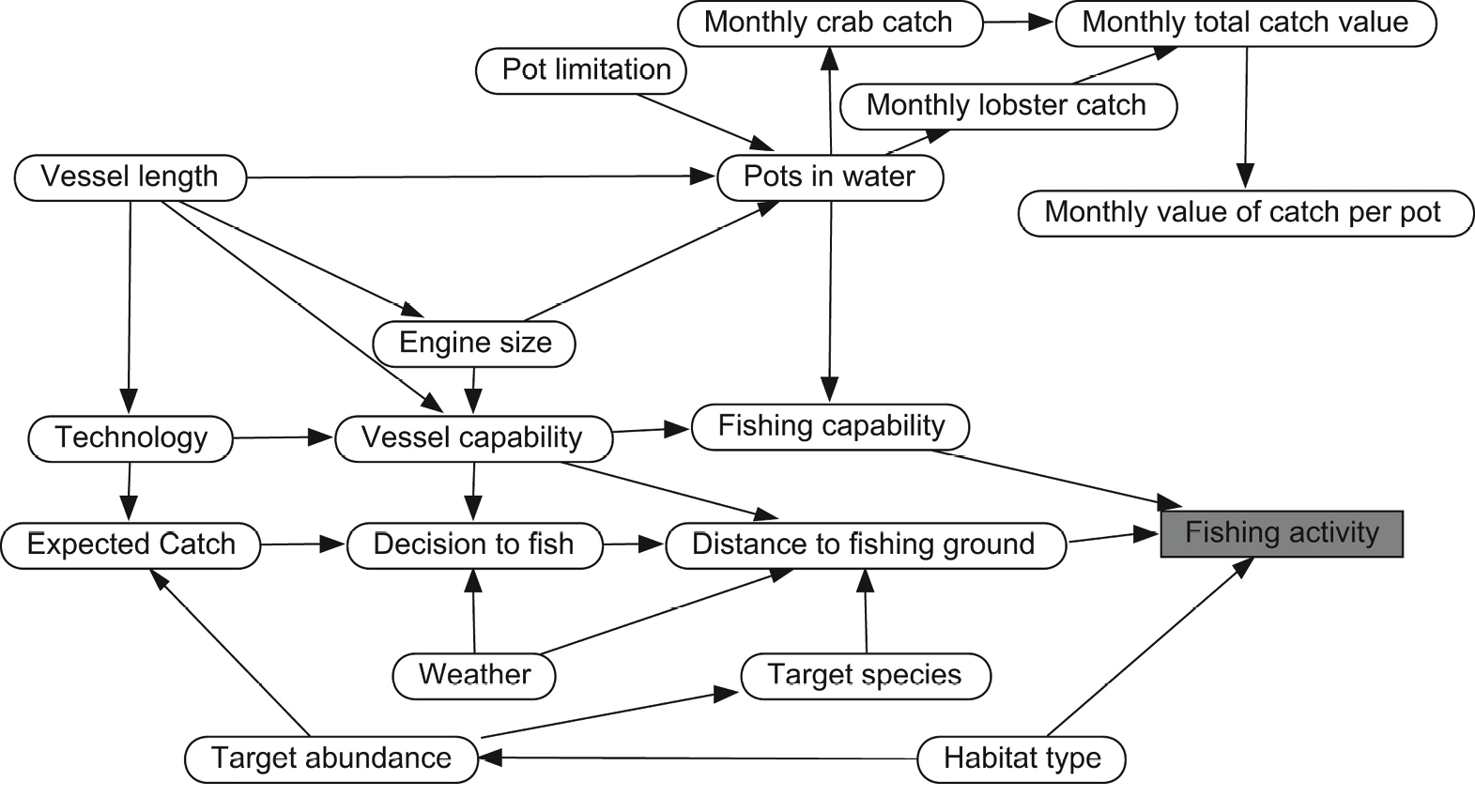
Figure 4.12 Inference diagram of the factors influencing pot-fishing activity along the Northumbrian coast, UK. (Source: Reprinted from Stephenson et al., 2018, with permission from Elsevier)

BNs can be used in evidence synthesis to contextualise evidence into a decision. A well conducted systematic review and meta-analysis can often only provide evidence for a small part of the full scope of a decision problem. For example, Carrick et al. (2019) asked the question ‘is planting trees the solution to reducing flood risks?’. Using a systematic review and meta-analysis they could only answer a lesser question about the effect of trees on stream flow. Flood risk is a wider issue and consists of many other factors that can influence the outcome. Using a BN to place the results of the systematic review into the full decision context, Carrick et al. (2019) were able to show the sensitivity of Flood Risk node to uncertainty in the other nodes in the network (Figure 4.13). This, in effect, allows one to quantify which uncertainties should be reduced first to get a better understanding of flood risk. These included, for example, infrastructure density (where roads and houses are placed on the landscape) and the capacity of reservoirs to slow down water flow into river catchments.

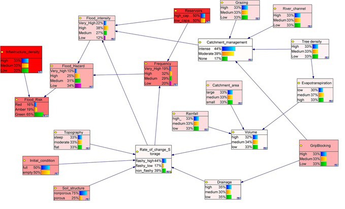
Figure 4.13 Bayesian networks are used to contextualise evidence for decision making. Here, ‘Flood Risk’ is dependent upon physical factors (e.g. soil structure, rainfall etc.) combined with human “interventions” such as storage dams (‘Reservoirs’) and changing upland drainage regimes (‘Grip Blocking’). An added benefit of using Bayesian networks is that the sensitivity of the focal node (‘Flood Risk’) to uncertainty in the other nodes in the network (darker shades of red indicate greater importance for reducing uncertainty). Reducing uncertainty in, for example, the ‘Reservoirs’ node will have a greater impact on our understanding of ‘Flood Risk’. Primary research could be targeted at these (darker red) nodes to reduce uncertainty in decisions about ‘Flood Risk’.The systematic review and meta-analysis of Carrick et al. (2019) represent a single node in the network (‘Tree density’) whilst all other nodes come from the literature. (Source: Carrick et al., 2019, © 2018 The Chartered Institution of Water and Environment Management (CIWEM) and John Wiley & Sons Ltd, reproduced with permission from John Wiley & Sons Ltd).

Bayesian networks can encompass decision nodes and utility nodes to make them explicit decision support tools (sometimes called Bayesian Decision Networks — see Nyberg et al. 2006). A decision node represents two or more choices that influence the values of outcome nodes. For example, the decision to mow or not to mow a grassland or to irrigate or not irrigate a crop could be included in the network. Utility nodes which show the value of an action in units of importance to the decision maker (this could be financial cost or expected change in the number of species) are often linked to these decision nodes to allow trade-offs between costs and benefits to be explored.

Several commercial packages (with limited free options) exist such as HUGIN, NETICA and GENIE and open source R packages such as bnlearn (Scutari, 2010) and caret (Kuhn, 2022) that can be used to develop BNs. Hybrid networks (combining continuous and categorical data) can now be developed using JAGs software (Plummer, 2003) through the R package Hydenet (Dalton and Nutter, 2019).

4.7.7 Evidence restatements

Policy decisions often need to be made in areas where the evidence base is both complex and heterogeneous (precluding formal meta-analysis) and highly contested. Evidence ‘Restatements’ seek to summarise the evidence base in a manner as policy neutral as possible while being clear about uncertainties and evidence gaps. If successful they can clarify the role of economic considerations, value judgements and other considerations in addition to the evidence base in the process of policy-making.

There are different ways to construct restatements and here we describe a model developed by the Oxford Martin School at Oxford University.

1. A topic is chosen after discussion with policy makers.
2. A panel of experts is then convened, typically from universities and research organisations.
3. A draft evidence summary is then prepared which takes the form of a series of numbered paragraphs written to be intelligible to a policy maker who is familiar with the subject but is not a technical expert. The summary is based on a systematic review of the literature and each statement is accompanied by an opinion on the strength of the evidence using a reserved vocabulary that varies between projects.
4. An extensive annotated bibliography is produced, linked to each paragraph, allowing policy makers access to the primary literature should they require further information.
5. The draft restatement is discussed paragraph by paragraph by the expert group and revised over several iterations.
6. This version is then sent out for review to a large group of people including other subject experts but also policy makers and interested parties (for example from the private sector and NGOs). They are asked to comment on the evidence itself, the assessment of the strength of the evidence, and also the aspiration that the restatement is policy neutral.
7. The restatement is revised in the light of these comments and the final version is drawn up after further iterations with the expert panel.
8. The restatement is submitted for publication to a journal (appearing as an appendix to a short ‘stub’ paper with the annotated bibliography as supplementary material online) where it receives a final review. Restatements are independently funded (by philanthropy).

Topics that have been the subject of restatements include the control of bovine TB in cattle and wildlife (Godfray et al., 2013) and the biological effects of low-dose ionising radiation (McLean et al., 2017). Other topics covered have included the effects of neonicotinoid insecticides on pollinators, landscape flood management, endocrine-disrupting chemicals, and control of Campylobacter infections.

Restatements have been popular with policy makers because (i) they strive to be policy neutral; (ii) they are conducted completely independently of the policy maker (important in areas of great contestation); (iii) they carry the authority of the expert panel and a scientific publication; and (iv) they are relatively brief and written to be understandable by policy makers. Their disadvantages include reliance on expert judgement (the heterogeneous evidence base precluding a more algorithmic approach) and the time and effort required of typically senior experts.

References

Adams, C.A., Fernández-Juricic, E., Bayne, E.M. et al. 2021. Effects of artificial light on bird movement and distribution: a systematic map. Environmental Evidence 10: Article 37, https://doi.org/10.1186/s13750-021-00246-8.

Ausden M., Sutherland W.J. and James R. 2001. The effects of flooding lowland wet grassland on soil macroinvertebrate prey of breeding wading birds. Journal of Applied Ecology 38: 320–38, https://doi.org/10.1046/j.1365-2664.2001.00600.x.

Back from the Brink. 2021. Looking After Spring Speedwell Veronica verna. Ecology and Conservation Portfolio (Salisbury: Plantlife), https://naturebftb.co.uk/wp-content/uploads/2021/06/Spring_speedwell_FINAL_LORES.pdf.

Boutin, C. and Harper, J.L. 1991. A comparative study of the population dynamics of five species of Veronica in natural habitats. Journal of Ecology 79: 199–221, https://doi.org/10.2307/2260793.

Buzan, T. 1974. Use Your Head (London: BBC Books).

Carrick, J., Abdul Rahim, M.S.A.B., Adjei, C., et al. 2019. Is planting trees the solution to reducing flood risks? Journal of Flood Risk Management 12(S2): e12484, https://doi.org/10.1111/jfr3.12484

Christie, A.P., Amano, T., Martin, P.A., et al. 2020a. The challenge of biased evidence in conservation. Conservation Biology 35: 249–62, https://doi.org/10.1111/cobi.13577.

Christie, A.P., Amano, T., Martin, P.A., et al. 2020b. Poor availability of context-specific evidence hampers decision-making in conservation. Biological Conservation 248: 108666, https://doi.org/10.1016/j.biocon.2020.108666.

Christie, A.P., Chiaravalloti, R.M., Irvine, R., et al. 2022. Combining and assessing global and local evidence to improve decision-making. OSF, https://osf.io/wpa4t/.

CMP. 2020. Conservation Standards, https://conservationstandards.org/about/.

Cramp, S. and Simmons, K.E.L. 1983. Handbook of the Birds of Europe, the Middle East and North Africa: The Birds of the Western Palearctic. Vol. III: Waders to Gulls (Oxford: Oxford University Press).

Dalton, J.E. and Nutter, B. 2020. HydeNet: Hybrid Bayesian Networks Using R and JAGS. R package version 0.10.11, https://cran.rproject.org/web/packages/HydeNet/index.html

Fedrowitz, K., Koricheva, J., Baker, S.C. 2014. Can retention forestry help conserve biodiversity? A meta-analysis. Journal of Applied Ecology 51: 1669–79,https://doi.org/10.1111/1365-2664.12289.

Gigerenzer, G. and Edwards, A. 2003. Simple tools for understanding risks: From innumeracy to insight. BMJ (Clinical research ed.) 327: 741–44, https://doi.org/10.1136/bmj.327.7417.741.

Green, R.E. 1986. The management of lowland wet grassland for breeding waders. Unpublished RSPB Report.

Green, R.E. 1988. Effects of environmental factors on the timing and success of breeding of common snipe Gallinago gallinago (Aves: Scolopacidae). Journal of Applied Ecology 25: 79–93, https://doi.org/10.2307/2403611.

Green, R.E., Hirons, G.J.M., and Cresswell, B.H. 1990. Foraging habitats of female common snipe Gallinago gallinago during the incubation period. Journal of Applied Ecology 27: 325–35, https://doi.org/10.2307/2403589.

Godfray, H.C.J., Donnelly, C.A., Kao, R.R., et al. 2013. A restatement of the natural science evidence base relevant to the control of bovine tuberculosis in Great Britain. Proceedings of the Royal Society B, Biological Sciences 280: 1634–43, https://doi.org/10.1098/rspb.2013.1634.

Hoodless, A.N., Ewald, J.A., and Baines, D. 2007. Habitat use and diet of common snipe Gallinago gallinago breeding on moorland in northern England. Bird Study 54: 182–91, https://doi.org/10.1080/00063650709461474.

Holton, N. and Allcorn, R.I. 2006. The effectiveness of opening up rush patches on encouraging breeding common snipe Gallinago gallinago at Rogersceugh Farm, Campfield Marsh RSPB reserve, Cumbria, England. Conservation Evidence 3: 79–80, https://conservationevidencejournal.com/reference/pdf/2230.

Iacona, G.D., Sutherland, W.J., Mappin, B., et al. 2018. Standardized reporting of the costs of management interventions for biodiversity conservation. Conservation Biology 32: 979–88, https://doi.org/10.1111/cobi.13195.

IPCC. 2005. Guidance Notes for Lead Authors of the IPCC Fourth Assessment Report on Addressing Uncertainties, July 2005 (Intergovernmental Panel on Climate Change), https://www.ipcc.ch/site/assets/uploads/2018/02/ar4-uncertaintyguidancenote-1.pdf.

Jensen, F.V. 2001. Causal and Bayesian networks. In: Bayesian Networks and Decision Graphs (New York: Springer), pp. 3–34.

Kuhn, M. 2022. Caret: classification and regression training. R package version 6.0-93, https://CRAN.R-project.org/package=caret.

Landuyt, D., Broekx, S., D’hondt, R., et al. 2013. A review of Bayesian belief networks in ecosystem service modelling. Environmental Modelling & Software 46: 1–11, https://doi.org/10.1016/j.envsoft.2013.03.011.

Malpas, L.R., Kennerley, R.J., and Hirons, G.J.M., et al. 2013. The use of predator-exclusion fencing as a management tool improves the breeding success of waders on lowland wet grassland. Journal for Nature Conservation 21: 37–47,https://doi.org/10.1016/j.jnc.2012.09.002.

Mason, C.F. and MacDonald, S.M. 1976. Aspects of the breeding biology of Snipe. Bird Study 23: 33–38, https://doi.org/10.1080/00063657609476482.

McLean A.R., Adlen, E.K., Cardis E., et al. 2017. A restatement of the natural science evidence base concerning the health effects of low-level ionizing radiation. Proceedings of the Royal Society B 284, 20171070, https://doi.org/10.1098/rspb.2017.1070.

Nabe-Nielsen, L.I., Reddersen, J., and Nabe-Nielsen, J. 2021. Impacts of soil disturbance on plant diversity in a dry grassland. Plant Ecology 222: 1051–63, https://doi.org/10.1007/s11258-021-01160-2.

Nyberg, J. B., Marcot, B.G., and Sulyma, R. 2006. Using Bayesian belief networks in adaptive management. Canadian Journal of Forest Research 36: 3104–16, http://wildlifeinfometrics.com/wp-content/uploads/2018/02/Nyberg_et_al_2006_Bayesian_Models_in_AM.pdf.

Plummer, M. 2003. JAGS: A program for analysis of Bayesian graphical models using Gibbs sampling. In: DSC 2003. Proceedings of the 3rd International Workshop on Distributed Statistical Computing, ed. by K. Hornik, et al., 124: 1–10, https://www.r-project.org/nosvn/conferences/DSC-2003/Drafts/Plummer.pdf.

Popotnik, G.J. and Giuliano, W.M. 2000. Response of birds to grazing of riparian zones. Journal of Wildlife Management 64: 976–82, https://doi.org/10.2307/3803207

Robson, B. and Allcorn, R.I. 2006. Rush cutting to create nesting patches for lapwings Vanellus vanellus and other waders, Lower Lough Erne RSPB reserve, County Fermanagh, Northern Ireland. Conservation Evidence 3: 81–83, https://conservationevidencejournal.com/reference/pdf/2231.

Salafsky, N., Boshoven, J., Burivalova, Z., et al. 2019. Defining and using evidence in conservation practice. Conservation Science and Practice 1: e27, https://doi.org/10.1111/csp2.27.

Salafsky, N., Irvine, R., Boshoven, J., et al. 2022. A practical approach to assessing existing evidence for specific conservation strategies. Conservation Science and Practice 4: e12654,https://doi.org/10.1111/csp2.12654.

Scutari, M. 2010. Learning Bayesian networks with the bnlearn R package. arXiv Preprint, https://doi.org/10.48550/arXiv.0908.3817.

Smart, J., Amar, A., O’Brien, M., et al. 2008. Changing land management of lowland wet grasslands of the UK: Impacts on snipe abundance and habitat quality. Animal Conservation 11: 339–51,https://doi.org/10.1111/j.1469-1795.2008.00189.x.

Spiegelhalter, D.J., Abrams, K.R., and Myles, J.P. 2004. Bayesian Approaches to Clinical Trials and Health-Care Evaluation, Vol. XIII (Chichester: John Wiley & Sons), https://doi.org/10.1002/0470092602.

Stewart, G. and Ward, J. 2019. Meta-science urgently needed across the environmental nexus: a comment on Berger-Tal et al. Behavioural Ecology 30: 9–10, https://doi.org/10.1093/beheco/ary155.

Stephenson, F., Mill, A.C., Scott, C.L., et al. 2018. Socio-economic, technological and environmental drivers of spatio-temporal changes in fishing pressure. Marine Policy 88: 189–203, https://doi.org/10.1016/j.marpol.2017.11.029.

Stewart, G.B., Mengersen, K., and Meader, N. 2014. Potential uses of Bayesian networks as tools for synthesis of systematic reviews of complex interventions. Research Synthesis Methods 5: 1–12, https://doi.org/10.1002/jrsm.1087.

Watt, A.S. 1971. Rare species in Breckland; their management for survival. Journal of Applied Ecology 8: 593–609, https://doi.org/10.2307/2402895.

White, T., Petrovan, S., Booth, H., et al. 2022. Determining the economic costs and benefits of conservation actions: A framework to support decision making. Conservation Science & Practice, https://doi.org/10.31219/osf.io/kd83v.

Wyden, P. 1980. The Bay of Pigs: The Untold Story (New York: Simon & Schuster).