
10. Public Spending for Future Generations: Recent Trends in EU Countries1
© 2022 Chapter Authors, CC BY-NC 4.0 https://doi.org/10.11647/OBP.0328.10
Introduction
Public investment, traditionally measured using the so-called gross fixed capital formation (hereinafter GFCF) of the public sector, decreased dramatically in the European Union (hereinafter EU) between 2010 and 2016, both as a percentage of GDP and in relation to the population, passing respectively from 3.7% to 2.7% of GDP and from approximately 1,000 to 800 euros per capita. The contraction of this category of expenditure, traditionally considered discretionary and more compressible by governments, is mainly due to the measures implemented to contain public expenditure (austerity) imposed in Europe following the global financial crisis and has therefore mainly affected the Mediterranean countries, which are traditionally characterised by high levels of public debt and low growth rates. As explained in Cerniglia and Saraceno (2021), there is only a partial recovery of public investment, which in 2019 reached 3% of GDP and approximately 890 euros per capita respectively, starting from 2017.
The use of the public sector GFCF (the so-called gross fixed investment) for the evaluation of government expenditure policies and the measurement of the latter’s impact not only on economic growth but also on the level of a country’s development and social and environmental prosperity, however, have been the subject of extensive institutional and academic discussions over the past few years. An example is the UN System of National Accounts, whose 2008 revision (UN 2009) expresses the need to consider the entire expenditure on Research and Development (hereinafter R&D) and Education in the GFCF.2 In the academic field, for example, Streeck and Mertens (2011) also include in the scope of their evaluation of public investment policies the so-called “soft investment”, i.e., public expenditure not accounted for as GFCF in R&D, Education, Active Labour Policies, and transfers to households. In fact, public sector GFCF expenditure is limited to the construction and maintenance of a country’s physical infrastructure (roads, railways, canals and bridges, machines used by the public sector). It can be easily noted that, first of all, the comparison of national policies carried out exclusively on the basis of this variable is made extremely complex by the latter’s dependence on both the geographical characteristics and the level of infrastructural development of each country.3 Secondly (and above all), we believe that the public sector GFCF does not include some items of expenditure which, although formally accounted for as “current” expenditure, decisively determine the public sector’s contribution to economic and social development and to the protection of a country’s environmental heritage, and must therefore be included in the evaluation of public expenditure policies and in the measurement of their effects on economic, social, and environmental indicators.4 The analysis of these categories of public expenditure is also motivated by some objectives and policies introduced at the European level such as, for example, the Next Generation EU, which require EU countries to spend a certain percentage of resources in projects aimed at promoting digital transition, scientific research, the green transition and social cohesion.
This chapter has two main objectives. First, we intend to contribute to the aforementioned debate by defining an innovative expenditure aggregate, which we have chosen to call Expenditure for Future Generations (hereinafter EFG) and which includes, in addition to the public sector GFCF, public contributions to investment by private companies (which, although they actually contribute to the creation and maintenance of a country’s private fixed capital stock, are not traditionally included in the GFCF), as well as primary current expenditure (hereinafter PCE) in some key sectors of public intervention, namely (i) Research and Development, (ii) Education, (iii) Environmental Protection, and (iv) General Economic, Commercial and Labour Affairs. In fact, it appears evident that (i) and (ii) contribute both to innovation in the industrial field and to the formation of human capital, which in turn have a positive impact on productivity and therefore on long-term economic growth (UN 2009). The PCE in Environmental Protection is mainly divided, within the European System of National Accounts, into the sub-functions management of solid and liquid waste, reduction of pollution, and protection of biodiversity and the landscape and, in our opinion, improves the quality of life of individuals. Finally, (iv) is linked to active employment policies, which increase employability prospects and therefore social inclusion (see, for example, Vooren et al. 2019). The dynamics of this innovative aggregate in the EU and for a group of “representative” countries of the geo-economic groups present within it will then be analysed and compared with those of the public sector GFCF. The second objective is to provide both European and national policymakers with innovative tools that allow them to evaluate (and, if necessary, modify) expenditure policies in European countries in relation to the EFG and economic categories (such as the GFCF) and the sectors comprising it. To this end we have defined three further variables, which we have called Comparative Advantage, Absolute Advantage, and Absolute Advantage Per Capita, which will make it possible to evaluate not only the performance in absolute terms (as a percentage of GDP and per capita) of the different countries of the EU in relation to the EFG and its components, but also in terms of the composition of public expenditure and therefore of expenditure priorities within the countries themselves. In particular, the analysis of these variables will allow us (i) to verify whether the EFG in the various countries is higher or lower than the EU as a whole (ii) to create a ranking of EU countries based on these variables and (iii) to look at trends in expenditure in EFG.
10.1 GFCF and EFG in the EU
10.1.1 From the GFCF to the EFG
The data relating to public expenditure used in our analysis are presented by the “Classification of the Functions of the Government” dataset (hereinafter COFOG), made available by Eurostat (and originally by OECD), which reports the public expenditure classified in functions5 (and sub-functions) of the government, the public entity that supports the expenditure (central and local administrations, and social security funds), as well as the economic category of expenditure (for example, GFCF, wages and salaries, interest on debt, intermediate and final consumption of the public sector). The data are presented in three main formats, namely in millions of euros, as a percentage of GDP, and as a percentage of total public expenditure. The geographical coverage includes all EU countries from 1995 to 2019.6 We define the EFG as the sum of the following economic categories of expenditure:
- GFCF in all functions of the state, generally defined as expenditure for (i) the construction of the physical infrastructure of a country; (ii) the purchase of capital goods used by the government; and (iii) to improve and maintain the existing capital stock (OECD 2009).
- Public Contributions to Investment: capital transfers in cash or in kind made by governments to other resident or non-resident institutional units in order to finance all or part of the costs of acquiring fixed assets (OECD 2009).
- PCE in the sectors of R&D, Education, Environmental Protection, and General Economic, Commercial and Labour Affairs.7 PCE is defined as the sum of (i) employee wages, (ii) intermediate consumption, (iii) subsidies, (iv) other current transfers, (v) social benefits other than social transfers in kind, and (vi) transfers that are social in nature—purchased market production (Lenzi and Zoppè 2020).
Finally, we define the Residual Primary Current Expenditure (hereinafter RPCE) as the PCE in the sectors not included in the EFG perimeter. It should be noted that the GDP deflator has been applied to the absolute values of all the variables in order to ensure the comparability of the series over time for the various countries.8
10.2 Trends in the EFG in the EU and Comparisons with the GFCF
In this section we focus on the temporal evolution of the EFG and the comparison of its dynamics with those of the GFCF. Figure 10.1 shows, respectively in the left and right columns, the GFCF and the EFG in relation to GDP (top) and per capita (bottom) for a subgroup of “representative” countries of the geo-economic subgroups that are part of (or were part of, in the case of the United Kingdom) the EU, or two “Mediterranean” countries (Italy and Spain), two Central European founding countries (France and Germany), a country belonging to the group of “new entrants” to the EU (Poland), a “Nordic” country (Sweden), the United Kingdom, and overall for the EU28 in the 2001–2019 period.9 Figure 10.2 shows, for the same countries and the same time interval, the GFCF (left) and EFG (right) as a percentage of the PCE and the RPCE, respectively. First of all, it can be noted that in some countries, namely Italy, Spain, Sweden, the United Kingdom, the EU as a whole and, to a lesser extent, Germany, GFCF and EFG follow rather similar dynamics. The only exceptions are France and, partially, Poland, where instead we observe at least a partial divergence between the two series. This result seems to indicate the existence of a shift between policies relating to gross fixed investment and other expenditure components included in the EFG.10 In particular, while the governments of the countries most affected by the measures implemented to contain public expenditure have contracted both the GFCF and the other components of the EFG following the imposition of austerity policies in response to the global financial crisis, those not affected by these measures did not reduce either of them (or even increased them, as in the case of Sweden).
It should be noted that Sweden is the country with the highest ratio of EFG to GDP and also to population, followed by France. Moreover, both countries show an increasing trend. The two countries also perform well in terms of GFCF. On the other hand, Poland, which is at the top of the ranking when we consider the ratio of GFCF to GDP, probably due to the EU funding for investment policies, does not show the same performance in terms of EFG. It is worth observing that Italy has a declining trend in the ratio of EFG to GDP reaching the last position at the end of the period.
With regards to the temporal dynamics of the variables relating to the EFG, it should first be noted that the EU value of the ratio between EFG and GDP first gradually increased, reaching a peak of 11.1% in 2009, and then gradually decreasing until 2018 (9.4%) and growing slightly in 2019. It should also be noted that, while the EFG per capita remains roughly constant during the analysis period, the ratio with the RPCE steadily decreases starting from 2006, reaching a minimum of 30.1% in 2018 and only partially recovering in 2019.
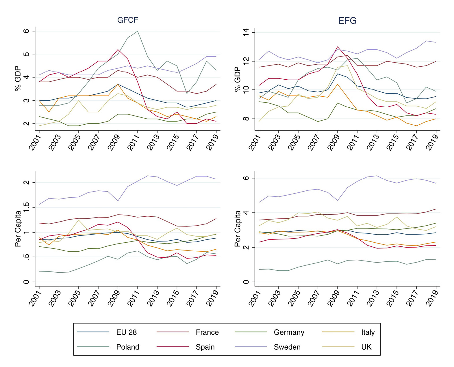
Fig. 10.1 GFCF (left) and EFG (right) as a percentage of GDP (top) and per capita (bottom) in thousands of euros, 2001–2019. Source: elaboration by the authors from Eurostat COFOG data.
The EFG follows profoundly different dynamics in the representative countries of the geo-economic groups identified above, which mainly depend on the austerity constraints introduced by the EU which have led, in some of them, to a substantial decrease in public expenditure on GFCF, traditionally considered more compressible with respect to current expenditure, and the other components of the EFG that, as explained above, are strongly correlated:
- Italy and Spain: in these countries, which are part of the group of the “Mediterranean” countries most affected by the measures to contain public spending, there is a substantial contraction in both the EFG and GDP ratio, which passes respectively from 10.4% and 13% in 2009 to 7.5% and 8.2% in 2017, and of the EFG per capita, which decreases from about 3,000 to just over 2,000 euros in 2017 and then begins to increase again only slightly. Furthermore, it can be noted that the relationship between EFG and RPCE is strongly reduced in both countries, respectively from 28.7% and 41.5% in 2009 to 20.4% and 27% in 2017, suggesting a recalibration of public expenditure at the expense of investment spending, which is traditionally considered more easily compressible and whose effects are observed with more delay by the voters (Cerniglia and Saraceno 2021).
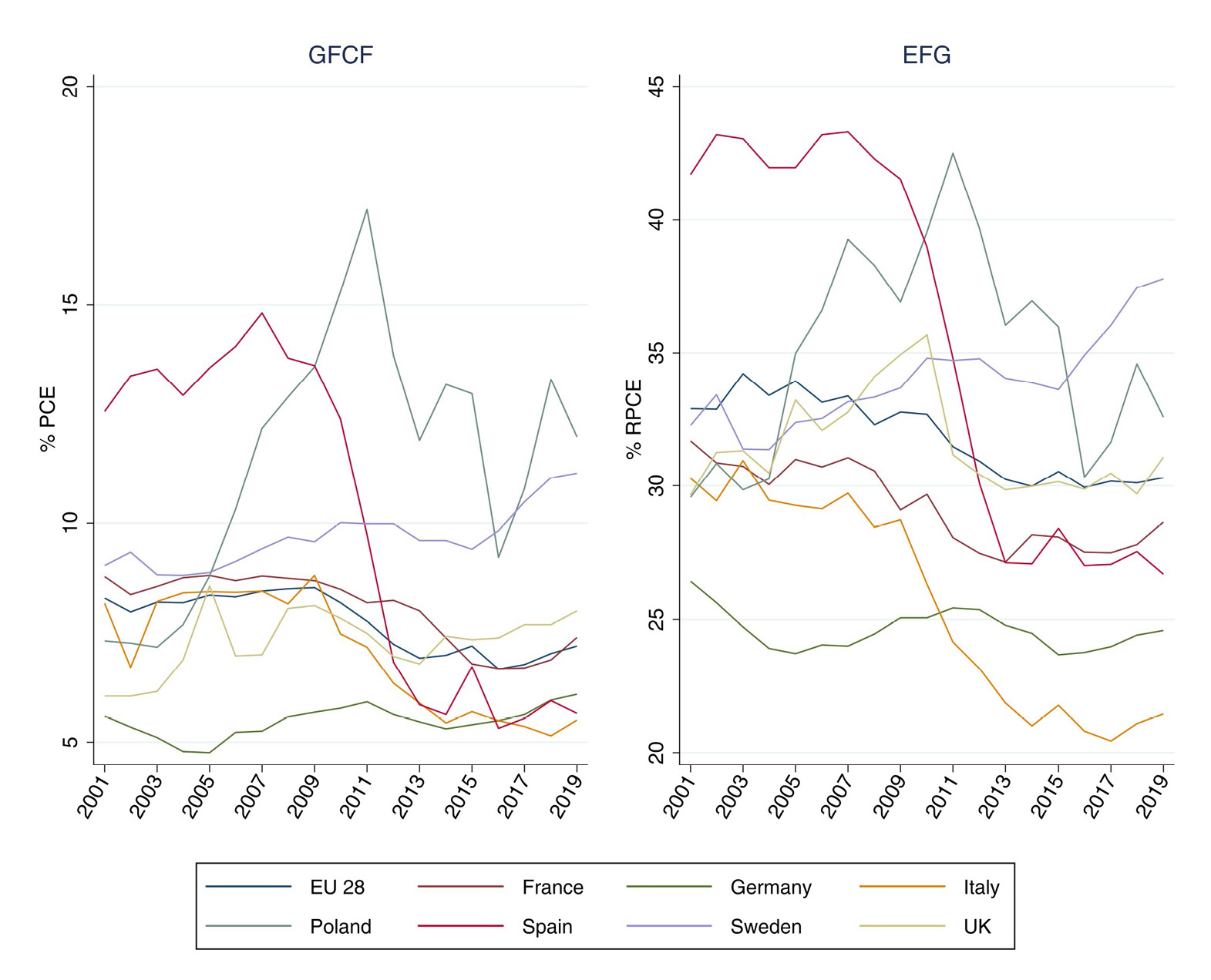
Fig. 10.2 GFCF (left) and EFG (right) as a percentage of public sector PCE and RPCE, 2001–2019. Source: elaboration by the authors from Eurostat COFOG data.
- France and Germany: France is characterised by similar dynamics to those of the Mediterranean countries in terms of GFCF on GDP and as a percentage of the PCR (but not of GFCF per capita), although much less pronounced, but the same cannot be said of EFG, which remains almost constant (if not slightly increasing) during the analysis period, and in any case always above the EU value. Nevertheless, it is possible to note a reduction in the ratio between EFG and RPCE, which goes from a maximum of 31% in 2010 to 27.5% in 2017. Germany, similarly to Italy, is characterised by an EFG decidedly below the EU value both in terms of GDP and RPCE in all the years analysed. First of all, it should be noted that the series for the two countries follow substantially similar trends up to 2009, with Germany characterised by an EFG that is lower than that of Italy both in terms of GDP and in relation to the RPCE. However, while in Italy the EFG has registered a very evident decline since 2010, the two ratios remain more or less constant in Germany. The problem of the low ratio of public investment to GDP in recent decades in Germany is analysed in Bardt et al. (2019). The authors identify as the main cause of these dynamics the erroneous forecasts of a decrease in the German working-age population and the consequent decrease in potential GDP growth, which then led to the fiscal consolidation measures introduced in 2009, in particular the “almost” breakeven budget (“Schuldenbremse”) introduced in the German constitution that limits the structural deficit of the public sector to 0.35% of GDP each year. Furthermore, some social reforms have shifted the tax burden of unemployment policies to municipalities, which in Germany also have the task of maintaining a whole series of infrastructures, such as roads and local public transport and schools. This further reduced the public investment rate of local authorities. As regards the EFG per capita, it is interesting to note once again how the historical series of Italy and Germany follow almost the same trends up to 2009, the year in which they start to diverge considerably. In particular, there is a slight increase in the EFG per capita in Germany, which reaches 3,400 euros in 2019.
- Poland: representative of the “New Entrants” countries in the EU in 2004, is characterised by an increase in all three relationships, also following the large amount of funds relating to the Cohesion Policy received after joining the EU. In particular, the ratios between EFG and GDP and between EFG and PCE reach their maximum, respectively 12.2% and 42.5%, in 2011, then decrease but remain stably above the EU value in 2019 (respectively 9.9% and 32.6%). Furthermore, the EFG per capita experiences a slow but almost constant growth trend. It is interesting to observe how, once the other components of the EFG are introduced into the analysis, the difference between per capita expenditure in Poland and in the Mediterranean countries increases (although it has been decreasing over the years), suggesting a lower priority of these sectors in the public expenditure policies of this country. The high ratio of EFG to GDP, accompanied by a low EFG per capita suggests, on the one hand, that Poland started in 2001 with a GDP per capita significantly lower than the EU value and, on the other hand, that the process of adjusting infrastructure of the country to European standards has been gradual but constant also in terms of per capita expenditure.
- Sweden: as in the other northern European countries not affected by the public debt containment measures introduced by austerity policies and traditionally characterised by efficient management of public resources, no decline is observed in the three ratios defined above, but rather an increase of the same during the analysis period. In particular, the ratios between EFG and GDP and between EFG and PCE rise respectively from 12.1% and 32.3% in 2001 to 13.3% and 37.8% in 2019, while the GFCF per capita, much higher than the EU as a whole for the whole period of analysis, increased from about 4,600 to 5,700 euros between 2001 and 2019.
- The United Kingdom: the ratio between EFG and GDP is below that of the EU for all the years analysed except those between 2008 and 2011. A similar trend can be observed for the relationship between EFG and PCE, although the latter converges at the EU value starting from 2011. Finally, the EFG per capita is always greater than the total EU value, although it approaches the latter towards the end of the period considered.
Figure 10.3 shows, for the selected countries and for the EU as a whole, the sum of public expenditure in relation to GDP for the different items that make up the EFG and the RPCE as an average for the years 2001–2007, 2008–2013, and 2014–2019. In particular, the EFG is divided into GFCF, Contributions to investments, Total Expenditure on Research and Development (GFLF and PCE), and PCE in the sectors of General Economic, Commercial, and Labour, Education, and Environmental Protection.11 An analysis of this graph allows us not only to analyse the composition of public expenditure (EFG or RPCE), but also to understand the weight of each component within EFG in the selected countries. Predictably, it can be seen that the RPCE represents the generally most relevant spending category in all countries, with a value in the EU in the three periods of respectively 30%, 32.7%, and 31.7% of GDP. It can be noted that the RPCE is higher than that of the EU overall in all three periods in France, Sweden, Germany, and Italy. The total EFG fluctuates between 9% and 10% in the EU in the three periods considered, and is, as already observed in Figure 10.1, higher than the EU figure for Sweden, France, and Poland.
Let us now move on to analyse the EFG components individually. First of all, it should be noted that, in addition to the GFCF, the PCE in Education represents (as widely expected) a very significant component of the EFG, equal to 4.73%, 4.75%, and 4.48% of EU GDP in the three periods analysed. It can also be observed that this ratio is lower in Spain, Germany, and Italy, which is the only country among the three in which the gap with the EU has widened over time. Regarding the total expenditure on Research and Development12 and the PCE on Environmental Protection, these two items represent a smaller percentage of the EFG in the countries analysed. In particular, EU expenditure on R&D is equal to 0.77% of GDP in the 2001–2007 period, and then grows to about 1% in the following two periods. It should be noted that the weight of this component is decidedly lower in the United Kingdom (although growing), Poland, Germany (which nevertheless reaches the EU value in the 2014–2019 period) and Italy, which, once again, sees the gap widening with the other countries over time. Similarly, the PCE in Environmental Protection grows from 0.46% to 0.5% between the first and last period overall in the EU, and is higher in Spain, Italy, France, and the United Kingdom. A similar argument applies to Public Contributions to Investments and to PCE in General Economic, Commercial and Labour Affairs, which represent residual categories in which the EU as a whole has spent between 0.5% and 0.7% of GDP respectively in the three periods analysed. It is interesting to note that, while the first item tends to decrease over time at the EU level and in most of the selected countries, an opposite trend is seen in France, where it increases from 0.55% to 0.8% of GDP between the first and the last period. Finally, as regards the PCE in General Economic, Commercial and Labour Affairs, the latter represents a substantial and growing component of the EFG especially for Sweden and France, where it reaches 1.45% of GDP between 2014 and 2019.
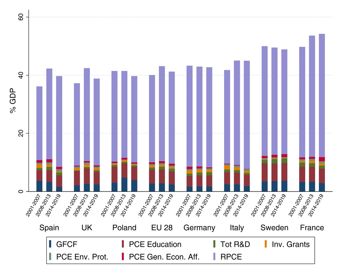
Fig. 10.3 Components of the EFG and RPCE, averages over the years 2001–2007, 2008–2013, and 2014–2019.
Source: elaborations by the authors from Eurostat COFOG data.
Finally, Figures 10.4 and 10.5 respectively show for all countries of EU 28 a scatterplot of the GFCF over GDP ratio on the PCE over GDP ratio (the two components of EFG) after the financial crisis (2010–2019) and a scatterplot of the change in the EFG over GDP ratio on the RPCE over GDP ratio from 2001–2009 to 2010–2019. The horizontal and vertical red lines in the figures represent the value of these two variables for EU 28 as a whole. From Figure 10.4 it can be observed that all Mediterranean countries (but Greece) plus Germany, Ireland and the UK are below the EU value in both components of the EFG, while all Nordic countries plus France, Netherlands, Luxembourg, and a few new entrants are above. It is also interesting to observe that most new entrants and Greece are above the European value in GFCF but not in PCE, probably due to the use of cohesion funds that focus especially on public investment.
When looking at Figure 10.5 it becomes apparent that all Mediterranean countries after the financial crisis have decreased the share of EFG over GDP while increasing the share of the other components of current expenditure. This is a concern to the extent that they seem to sacrifice expenditure for future generations probably due to the short-run attitude of their governments. Conversely, all Nordic countries and most European continental countries have increased (or maintained at an even level) the EFG over GDP ratio. Finally, many new entrants have decreased the EFG while increasing RPCE shares (although less than the EU average), probably also due to the convergence of their stock of physical capital to European standards.
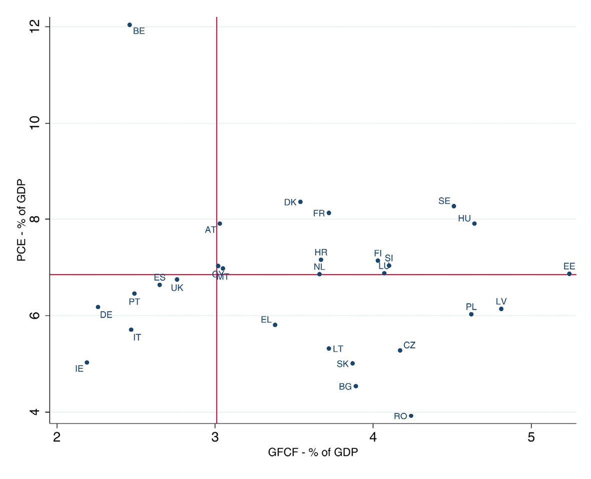
Fig. 10.4 PCE over GDP ratio and GFCF over GDP ratio for EU countries averages over the years 2010–2019.
Source: elaborations by the authors from Eurostat COFOG data.
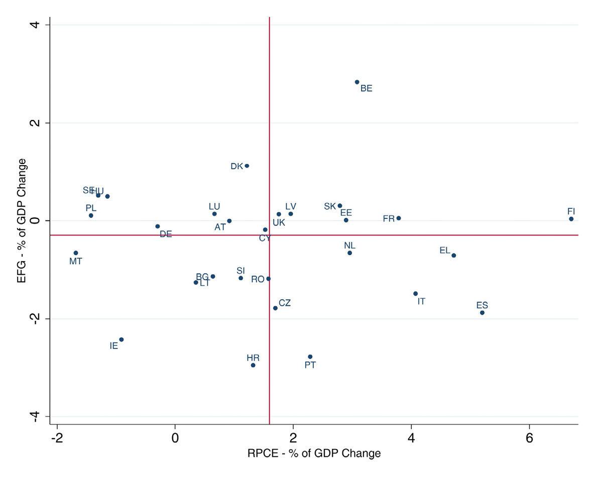
Fig. 10.5 Change in EFG over GDP and change in RPCE over GDP between 2001–2009 and 2010–2019.
Source: elaborations by the authors from Eurostat COFOG data.
10.3. Comparative and Absolute Advantage: International Comparisons
10.3.1 Definition of Variables
In the previous paragraph we defined a new aggregate, the EFG, which we believe more accurately captures the vast range of national public expenditure policies aimed at economic and social development and progress, and at the environmental protection of a country. We now focus on the definition of some “advantage” indicators that we believe can be of support to policymakers in evaluating and, if necessary, adjusting these expenditure policies. In order to compare the EFG of the various European countries we introduce, in particular, three indices, called (i) Comparative Advantage (hereinafter CA), (ii) Absolute Advantage (hereinafter AA), and (ii) Absolute Advantage Per Capita (hereinafter AA per capita). While indices (ii) and (iii) allow us to verify whether each of the EU countries in a given year has experienced a ratio between EFG and, respectively, GDP and population that is lower or higher than the EU as a whole, (i) is a measure of the country’s specialisation in this expenditure component with respect to the other components.
In particular, the CA, similar to the index developed by Balassa (1965; 1989), which measures the export specialisation of countries, is defined as the ratio between (i) the EFG divided by the total expenditure of the public sector in the generic country i in the considered year t and (ii) the EU EFG as a whole divided by total public sector expenditure in the EU in considered year t. Note how this index, which allows us to analyse the expenditure priorities of EU countries in terms of its composition, is greater (less) than 1, and therefore takes the form of a comparative advantage (disadvantage) for a country if the percentage of EFG expenditure compared to the total in the year considered is greater (less) than that of the EU as a whole:
We define AA as the difference between the EFG on GDP in generic country i in considered year t minus the EFG on overall EU GDP in the same year. Obviously, if this difference is greater (less) than zero, country i will have an absolute advantage (disadvantage) in the year considered:
Finally, the AA per capita is defined in a similar way as the difference between the EFG on the population residing in generic country i in year t minus the EFG on the total EU population (in thousands of euros) in the same year. Again, a positive (negative) value implies that generic country i has a higher (lower) EFG than the EU as a whole in the year. Formally:
10.3.2 Indicators of Advantage in the EU: Evolution
First of all, note that there is a decidedly positive correlation between AA and CA and, although lower, between AA and AA per capita (0.57 and 0.29 respectively). The correlation between AA per capita and CA is instead extremely close to zero (0.002), suggesting that the two variables are not correlated when we consider the whole sample. The latter result seems to indicate that the specialisation of countries in the EFG does not necessarily coincide with a high EFG per capita.
Figures 10.6, 10.7, and 10.8 show the evolution, respectively, of the CA, AA, and AA per capita in all EU28 countries in the 2001 to 2019 period. It is useful to divide the countries again into the groups already identified above:
- “Mediterranean” countries: Italy is characterised by CA below 1 and negative AA and AA per capita in all the years analysed. It should be noted that these disadvantages tend to worsen significantly during the period analysed, with a particularly evident collapse starting from 2010 and, subsequently, substantial stability. A similar dynamic can be observed for Greece, although the latter starts in 2001 in line with the EU in terms of CA and AA and, after experiencing a sharp decline in spending following the austerity measures, returns to pre-crisis levels in 2018. It should also be noted that Greece is characterised by a constant negative AA per capita and affected by a marked decrease starting from 2009. Spain and Portugal instead have a very positive CA and AA (although decreasing for Portugal) until 2009, the year from which the aforementioned cost containment measures come into force. However, it should be noted that Portugal, and for almost all the years of analysis, Spain, are affected by an EFG per capita that is lower than that of the EU as a whole. Ireland, one of the countries most exposed to the European sovereign debt crisis and subjected to severe austerity measures, follows partially comparable dynamics. In particular, a decidedly increasing absolute disadvantage can be observed starting from 2009, accompanied by a substantial decrease in the CA between 2008 and 2010. The latter returns in any case greater than 1 in 2015 (and increasing), while the AA per capita is always positive between 2001 and 2019.
- “Nordic” countries: it can be noted that Denmark, Finland, and Sweden have a generally positive and increasing AA and AA per capita in the analysis period. Note, however, that while Sweden is characterised by a consistently positive and strongly increasing CA, Denmark experiences a slight comparative disadvantage until 2011 and then follows the same dynamics as Sweden. Finally, in Finland, the CA is only initially positive, but then converges to 1 and becomes even slightly lower starting from 2015. Belgium, France, and Austria, even if not strictly belonging to this geographical aggregation, are affected by similar dynamics. Belgium, in particular, is characterised by a very strong increase in all three variables analysed starting from 2006, while France and Austria have a CA around unity for the entire analysis period, accompanied by positive and growing AA and AA per capita. Finally, the Netherlands, although experiencing substantial advantages in relation to EFG, is affected by a slight but steady decrease in CA and AA over the years.
- “New Entrants”: the countries that entered the EU after 2004, i.e. the Baltic republics (Estonia, Latvia, and Lithuania), the Czech Republic, Poland, Romania, Slovenia, Slovakia, Bulgaria, and Croatia, are characterised in most cases by strong comparative and absolute advantages. However, they are generally accompanied by negative AA per capita in all the years analysed. It is interesting to note that Romania, the Czech Republic, and Lithuania have comparative advantages even in the face of absolute negative AAs, suggesting that countries pay particular attention to the EFG, probably also thanks to cohesion policies.
- Germany and the UK: both countries have negative AA (apart from the UK between 2008 and 2010) throughout the analysis period. However, the United Kingdom has a slightly positive AA per capita in this time interval, while the latter is negative for Germany until 2008. Furthermore, Germany is characterised by a significant comparative disadvantage, although the latter tends to decrease over time.
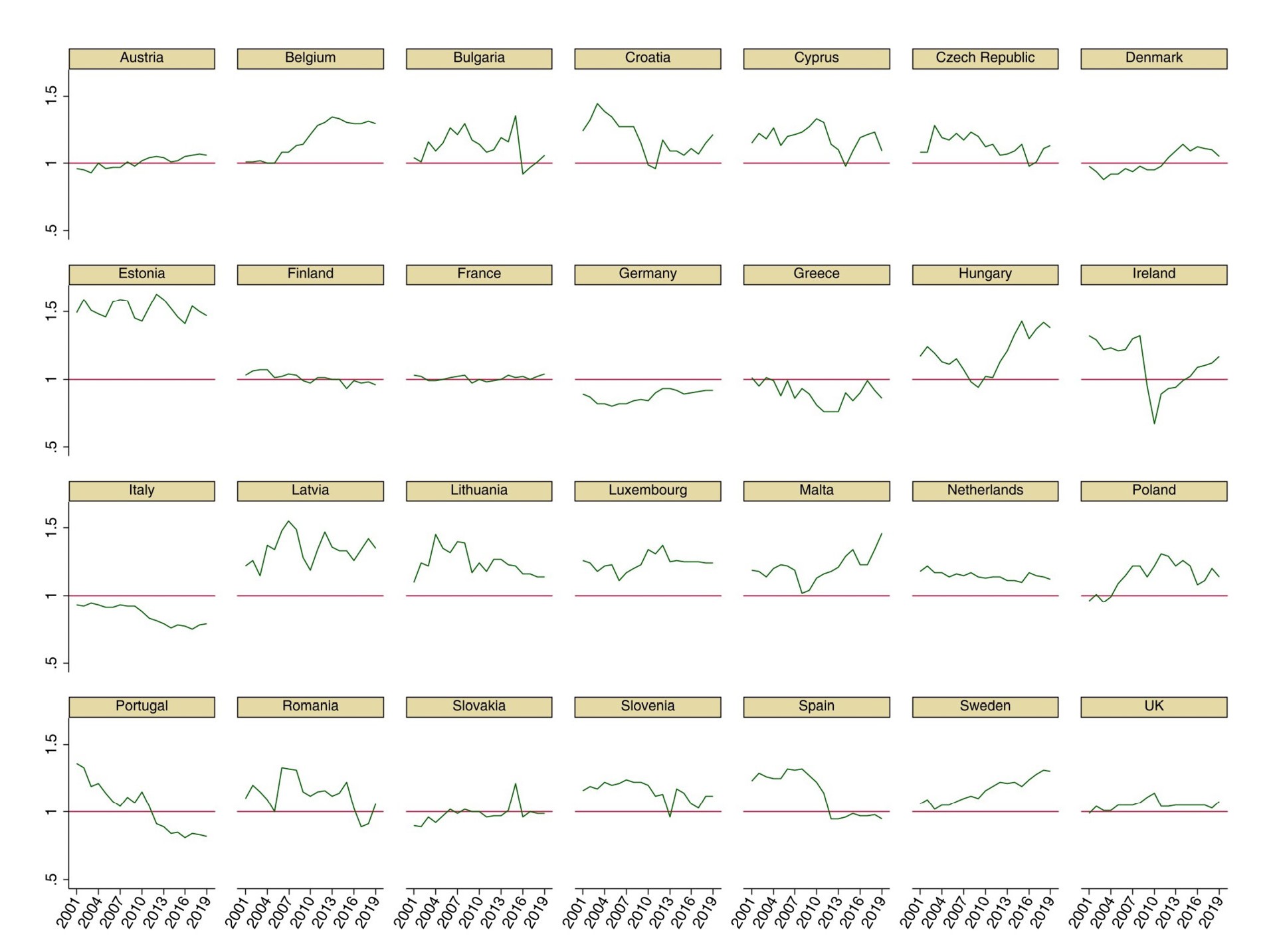
Fig. 10.6: CA in EU28 countries in the EFG, 2001–2019.
Source: elaborations by the authors from Eurostat COFOG data.
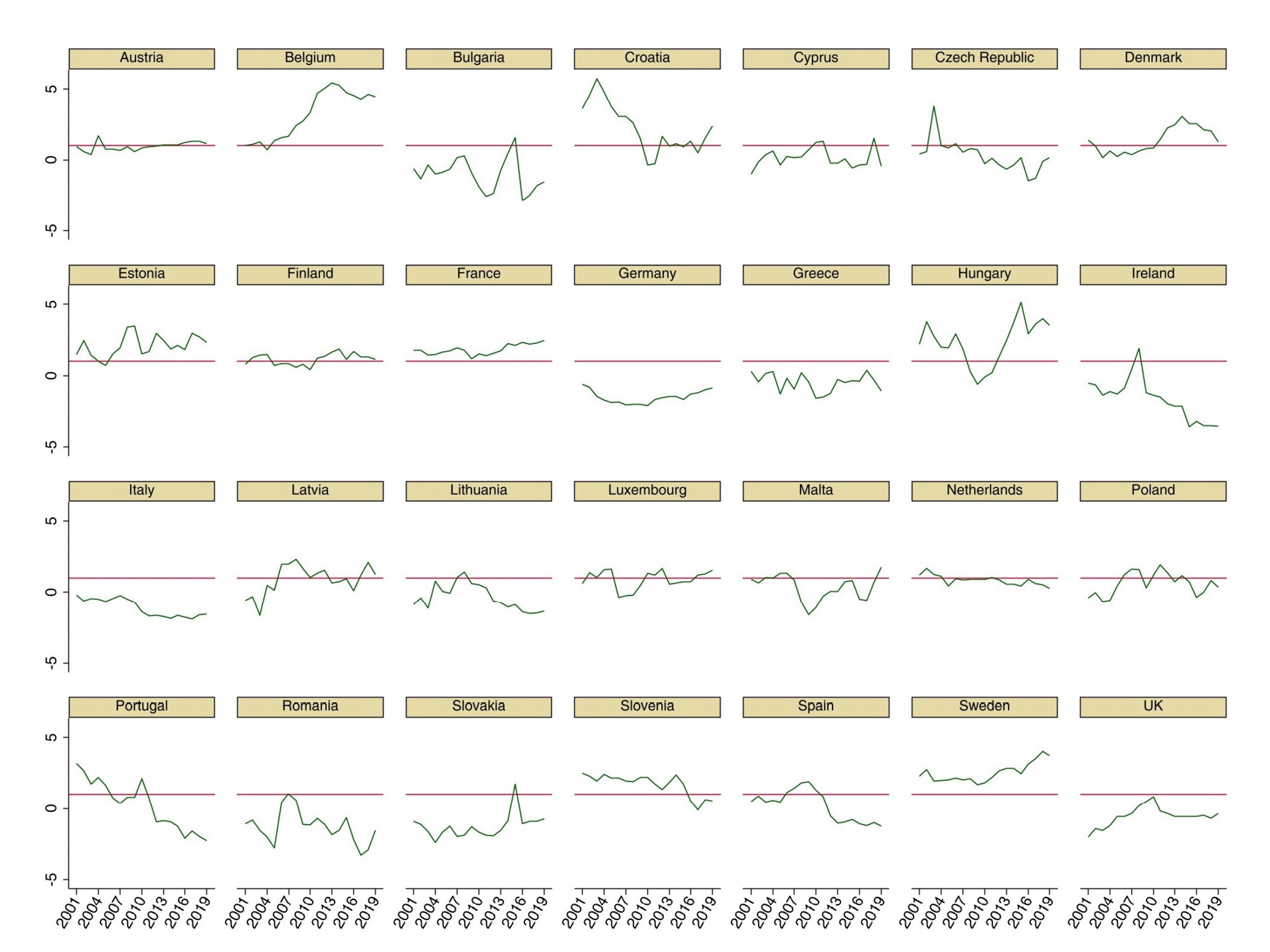
Fig. 10.7: AA in EU28 countries in the EFG, 2001–2019.
Source: elaborations by the authors from Eurostat COFOG data.
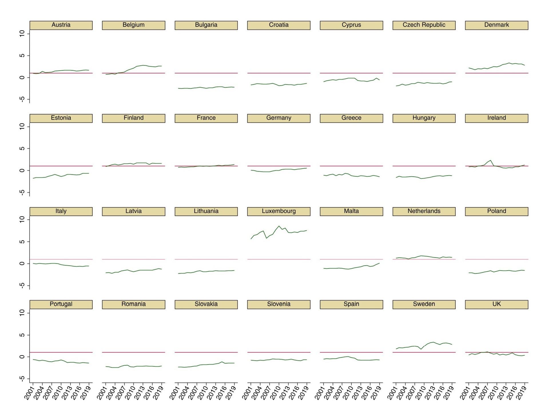
Fig. 10.8: AA per capita in EU28 countries in the EFG, 2001–2019.
Source: elaborations by the authors from Eurostat COFOG data.
Finally, Table 10.1 shows the CA, AA, and AA per capita of the countries selected in the 2001–2019 period (for the sake of brevity) in relation to the aggregates that make up the EFG , or GFCF , Current Expenditure on General Economic, Commercial, and Labour Affairs, Education, Environmental Protection, Total Expenditure on Research and Development, and Public Contributions to Investment. A synthetic index is also presented for the Primary Current Expenditure in all the key sectors that make up the EFG (thus excluding the Public Contributions to Investment).
We believe that the use of these metrics, taken both individually and as a whole, can provide a valid guide to public decision-makers at the national level in order to verify the past performance of national public policies, but also to modify them, if deemed appropriate and possible, given the domestic and European political constraints on expenditure in the future. The CA, in particular, provides an extremely useful indicator even in the presence of constraints on public expenditure, and provides an incentive to rebalance the latter in favour of expenditure items aimed more at a country’s economic and social development.
Table 10.1 Absolute advantage, absolute advantage per capita (in thousands of euros) and comparative advantage for the selected EU28 countries in the components of the EFG, averages over the years 2001–2019.
|
Country |
Index |
GFCF (R&D included) |
PCE Key sectors |
PCE General Economic, Commercial, and Labor Affairs |
PCE Environmental Protection |
PCE Education |
Total expenditure in R&D |
Public Contributions to Investment |
|
France |
CA |
1.05 |
0.98 |
1.21 |
1.1 |
0.94 |
1.18 |
1.01 |
|
AA |
0.73 |
0.88 |
0.27 |
0.14 |
0.47 |
0.35 |
0.11 |
|
|
AA PC |
0.33 |
0.33 |
0.1 |
0.05 |
0.18 |
0.13 |
0.04 |
|
|
Germany |
CA |
0.72 |
0.87 |
1.03 |
0.94 |
0.84 |
1.04 |
1.62 |
|
AA |
-0.93 |
-0.91 |
0 |
-0.04 |
-0.87 |
0.01 |
0.35 |
|
|
AA PC |
-0.14 |
-0.36 |
0 |
-0.02 |
-0.34 |
0 |
0.14 |
|
|
Italy |
CA |
0.86 |
0.79 |
0.26 |
1.14 |
0.83 |
0.88 |
1.55 |
|
AA |
-0.32 |
-1.03 |
-0.47 |
0.09 |
-0.65 |
-0.08 |
0.37 |
|
|
AA PC |
0.04 |
-0.36 |
-0.16 |
0.03 |
-0.23 |
-0.03 |
0.13 |
|
|
Poland |
CA |
1.44 |
1.09 |
0.86 |
0.59 |
1.17 |
0.59 |
0.71 |
|
AA |
1.03 |
0.05 |
-0.13 |
-0.22 |
0.4 |
-0.41 |
-0.21 |
|
|
AA PC |
-0.64 |
0.01 |
-0.02 |
-0.03 |
0.05 |
-0.05 |
-0.03 |
|
|
Spain |
CA |
1.24 |
1.07 |
1.62 |
1.63 |
0.93 |
1.16 |
1.39 |
|
AA |
0.35 |
-0.24 |
0.29 |
0.23 |
-0.76 |
0.04 |
0.15 |
|
|
AA PC |
-0.01 |
-0.07 |
0.08 |
0.07 |
-0.22 |
0.01 |
0.04 |
|
|
Sweden |
CA |
1.29 |
1.17 |
1.22 |
0.7 |
1.21 |
1.41 |
0.29 |
|
AA |
1.25 |
1.57 |
0.21 |
-0.12 |
1.48 |
0.48 |
-0.42 |
|
|
AA PC |
0.7 |
0.8 |
0.11 |
-0.06 |
0.75 |
0.24 |
-0.21 |
|
|
The UK |
CA |
0.95 |
1.12 |
0.71 |
1.36 |
1.15 |
0.46 |
1.46 |
|
AA |
-0.46 |
0.05 |
-0.23 |
0.11 |
0.17 |
-0.53 |
-0.21 |
|
|
AA PC |
-0.07 |
0.02 |
-0.1 |
0.05 |
0.08 |
-0.24 |
0.09 |
Source: elaborations by the authors from Eurostat COFOG data.
10.4 Conclusions and Policy Considerations
In this chapter we have proposed a new aggregate for comparing the “quality” of public expenditure across countries. While there is a large literature emphasising the importance of public investment with respect to public current expenditure, with the first considered to be more conducive to economic growth than the latter, we believe that public investment alone does not capture the contribution of the public sector to economic and social development and to the protection of the environment. We have therefore considered a larger aggregate which we have defined as Expenditure for Future Generations (EFG) and which includes, in addition to the public sector GFCF, public contributions to investment by private companies as well as primary current expenditure in some key sectors of public intervention, namely (i) Research and Development, (ii) Education, (iii) Environmental Protection, and (iv) General Economic, Commercial and Labour Affairs. The analysis of this aggregate is more in line with the objectives and policies introduced at the European level in the Next Generation EU, which include among its priorities sustainable development and social cohesion. We have shown that, particularly after the financial crisis, countries with high levels of debt have also strongly reduced this component of overall public expenditure when they have not cut the overall share of public expenditure over GDP.
Overall, we are convinced that governments should focus on indicators of public expenditure that are consistent with the long-term objectives of sustainable development. Since this does not seem to have been the case in many countries (Italy is a typical example), such an approach could be taken at the European level. While this may require an extended “golden rule”, the difficulty faced so far in following this path suggests that it is unlikely that it will be adopted in the future. Alternative policies might include a larger flexibility in the application of the European fiscal rules for these types of expenditures and/or even just a monitoring of the evolution of EFG across countries and over time, since indicators on their own have the merit of raising the attention towards the variables that they capture.
We are aware that the indicator we propose is very tentative and can certainly be improved, but we think that we should go beyond the simple distinction between GFCF and current government expenditure consistently with a shift in the focus from GDP to broader concepts of sustainable development. Future studies may try to test whether EFG and/or their sub-components positively impact GDP and/or multidimensional measures of sustainable development.
References
Balassa, B. (1965) “Trade Liberalization and ‘Revealed’ Comparative Advantage”, The Manchester School of Economic and Social Studies 33: 92–123.
Balassa, B. (1989) “’Revealed’ Comparative Advantage Revisited”, in B. Balassa (ed.), Comparative Advantage, Trade Policy and Economic Development, New York: New York University Press, pp. 63–79.
Cerniglia, F. and F. Saraceno (2020) A European Public Investment Outlook, Cambridge: Open Book Publishers, https://doi.org/10.11647/OBP.0222.
Agenzia per la Coesione Territoriale, Nucleo di Verifica e Controllo, Area 3 Monitoraggio dell’attuazione della politica di coesione e Sistema Conti Pubblici Territoriali (2020) Analisi degli Investimenti Pubblici. Dati, Indagine Diretta ai Responsabili Unici del Procedimento e Casi di Studio. Roma: CPT Temi, https://www.agenziacoesione.gov.it/wp-content/uploads/2021/03/CPT_InvestimentiPubblici-1.pdf.
Eurostat (2019) Manual on Sources and Methods for the Compilation of COFOG Statistics. Luxembourg: Publications Office of the European Union, https://ec.europa.eu/eurostat/documents/3859598/10142242/KS-GQ-19-010-EN-N.pdf/ed64a194-81db-112b-074b-b7a9eb946c32?t=1569418084000.
European Commission (2022) Cohesion in Europe towards 2050—Eighth Report on Economic, Social and Territorial Cohesion. Luxembourg: Publications Office of the European Union, https://ec.europa.eu/regional_policy/sources/docoffic/official/reports/cohesion8/8cr.pdf.
Lenzi, F. S. and A. Zoppé (2020) Composition of Public Expenditures in the EU. Brussels: European Parliamentary Research Service (EPRS), https://www.europarl.europa.eu/RegData/etudes/BRIE/2019/634371/IPOL_BRI(2019)634371_EN.pdf.
OECD (2015) Frascati Manual 2015: Guidelines for Collecting and Reporting Data on Research and Experimental Development. Paris: OECD Publishing, https://www.oecd-ilibrary.org/science-and-technology/frascati-manual-2015_9789264239012-en.
OECD (2010), National Accounts at a Glance 2009. Paris: OECD Publishing, https://doi.org/10.1787/9789264067981-en.
Streeck, W. and Mertens, D. (2011) “Fiscal Austerity and Public Investment: Is the Possible the Enemy of the Necessary?” MPIfG Discussion Paper 11/12, Max Planck Institute for the Study of Societies, https://papers.ssrn.com/sol3/papers.cfm?abstract_id=1894657.
United Nations et al. (2009) System of National Accounts 2008. New York: United Nations, https://unstats.un.org/unsd/nationalaccount/docs/SNA2008.pdf.
Vooren, M., Haelermans, C., Groot, W, Maassen van den Brink, H. (2019), “The Effectiveness of Active Labor Market Policies: A Meta-Analysis”, Journal of Economic Surveys 33(1): 125–49, https://onlinelibrary.wiley.com/doi/epdf/10.1111/joes.12269.
1 This work has benefited from a postdoctoral grant provided by the Territorial Public Accounts (CPT) of the Agency for Territorial Cohesion.
2 A similar need is expressed by the Italian Territorial Cohesion Agency (CPT 2020).
3 For example, a low expense for the construction of new highways in a country like Germany could be justified by the presence of an already highly developed motorway infrastructure.
4 As specified in Streeck and Mertens (2011), “it would be necessary to focus attention on a different kind of public investment that is more important for post-industrial societies: the so-called ‘light investment’ which can be defined as those types of public expenditure that have as their objective that of creating the conditions for increasing the prosperity and sustainability of a post-industrial knowledge society.”
5 The intervention sectors defined in COFOG are General Public Services, Defence, Economic Affairs, Environmental Protection, Construction and Community Services, Healthcare, Recreation, Culture and Religion, Education, and Social Protection. Each sector is divided into a series of specific subsectors.
6 It should be noted that the time series for the United Kingdom is no longer present in the Eurostat dataset starting from 2021. Furthermore, some of the entries in the COFOG dataset are only available starting from 2001.
7 This sub-function of the “Economic Affairs” function is made up of the sub-items “General Economic and Commercial Affairs” and “General Labour Affairs”. The first sub-item includes, among other functions, the formulation and implementation of general economic and commercial policies, as well as the management and support of institutions that deal with patents, trademarks, and copyrights. The second includes general labour policies and policies aimed at increasing employability and reducing the unemployment rate.
8 In order to ensure series comparability between GFCF and EFG we have chosen not to use the deflator of the GFCF.
9 The choice of the 2001–2019 time interval for the analysis carried out derives from the lack of data on public expenditure on research and development from 1995 to 2000.
10 The correlation between FLCF and the sum of the other components of the SGF is positive for Italy (0.77), Spain (0.66), Sweden (0.69), the United Kingdom (0.65), Germany (0.12), and the EU 28 as a whole (0.52). This correlation is instead strongly negative for France (-0.7) and partially for Poland (-0.31).
11 Note that R&D expenditure, presented separately, has been subtracted from the GFCF and PCE in key areas.
12 Note that the data for R&D expenditure present in the COFOG dataset are not perfectly superimposable on those of the two datasets traditionally used for the analysis of this expenditure, namely GERD and GBARD, as explained in OECD (2015). While COFOG and GERD expenditure data are based on the national accounts principle, GBARD data are recorded on a budgetary basis. In addition, GERD data are reported along the “R&D performance sectors” and separately for the government sector and higher education. Finally, the GBARD data for some countries do not include local government expenditure. In any case, the correlation between COFOG and GERD/GBARD data is very high, 0.84 and 0.79 respectively. It is also important to underline that R&D spending does not constitute a separate sector in COFOG but is present as a sub-item in every function of the state.