13. Spatial Movement of Sound Vectors
Ambrosio Salvador Rodríguez Lara
© 2024 Ambrosio Salvador Rodríguez Lara, CC BY-NC 4.0 https://doi.org/10.11647/OBP.0390.15
Introduction
In the field of physics, a vector is a quantity that has both magnitude and direction. In this chapter, I propose the concept and definition of what I shall call a “sound vector” in acoustic space, understood as the space of auditory phenomena within which we characterize sounds as high or low, simultaneous or sequential, and so on. I also explain that rhythmic-melodic movement meets this definition. In musical instruments such as the harp, the marimba, or the piano, when a melody is played, sound vectors are projected simultaneously over the acoustical space as well as over the physical space of the instrument. By using technological resources to synchronize several acoustic sources, not only is it possible to obtain a projection of sound impulses in wider spaces but also to model that projection on particular physical spaces, just as rhythmic-melodic sequences are modeled within the acoustic space. However, unlike the instruments mentioned above, in which each pitch is located only in one place, we find that, when using different sound sources, the possibilities of distribution regarding each sonorous aspect of the impulse—pitch, rhythm, dynamics, stress, timbre, etc.—get remarkably diversified. All this, in turn, leads to a great expressive flexibility. In this discussion, electroacoustic sources and means are excluded.
Sound vectors are classified in continuous and non-continuous displacement impulses. Some of my compositions, and those of other composers that show non-continuous displacement impulses, are presented as examples. In addition, I propose some compositional possibilities for this type of impulses. It is interesting to consider impulses with relatively fast speed over the physical space, like a glissando on the harp or the piano, and the impression that these produce of a near cancelation of both the physical and the acoustical spaces between the sources. Sound vectors are a resource of great expressiveness.
Definition of a Sound Vector
The definition that I propose for the term “sound vector” is the following: a sound impulse that moves in the audible frequency range—or acoustical space—with a determined speed and direction. Speed and direction are the two basic properties of a sound vector. We can define speed in this context as the number of events that occur within a certain duration. This definition allows for correspondence with the field of physics, where speed is a scalar magnitude and velocity is a vector, i.e., it has magnitude and direction in physical space.
In string instruments and keyboards, such as the piano, the harp, the marimba, or the vibraphone, sound impulses, through rhythmic-melodic movement, form simultaneously a trajectory in physical space that moves parallel to the rhythmic-melodic trajectory: a sound vector in acoustical space behaves as a sound vector in physical space, sharing the properties of speed and direction of the sound impulses. On the other hand, the continuous repetition of a sound event on these instruments does not move in the acoustic space or the physical space. Under such conditions, the sound event has a speed, but since it has no direction in the acoustical nor physical spaces, it is not considered a sound vector. Nevertheless, as explained below, textures can be organized so that repeated events do form sound vectors in physical space through the interaction of synchronized, fixed sources in a given space to produce sound impulses with speed and direction.
As emphasized above, I am referring exclusively to acoustic sources, so every electroacoustic source or means is excluded.
Classification of Sound Vectors
Sound vectors can be classified into two categories: continuous displacement sound vectors and non-continuous displacement sound vectors.
Continuous Displacement Sound Vectors
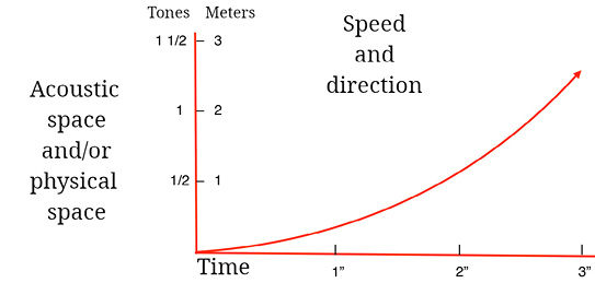
Fig. 13.1 Continuous displacement sound vectors are impulses that travel through all points in physical space, such as a glissando. Figure created by author (2022).
This kind of sound impulse comes from a source that can move continuously and travel through all points in a space, either physical or acoustical. A well-known example that encompasses both spaces simultaneously is the siren of an ambulance, which travels as a glissando through a certain extension of the acoustical space and moves continuously in physical space to a listening point and then away from it. When moving closer with a certain speed, the Doppler effect is produced: the values of frequency and intensity grow; the sound reaches a peak in frequency and intensity when the ambulance passes near the listener. After, when it moves away, the frequency and the intensity drop simultaneously.
Another example of a continuous displacement impulse in the acoustical space is a glissando in a string instrument like the violin, or in an air column like the trombone, or the human voice.
A different case of continuous displacement of sources in physical space, though much slower, can be observed in religious processions, marches, and military parades, even in funeral processions.
Non-continuous Displacement Sound Vectors
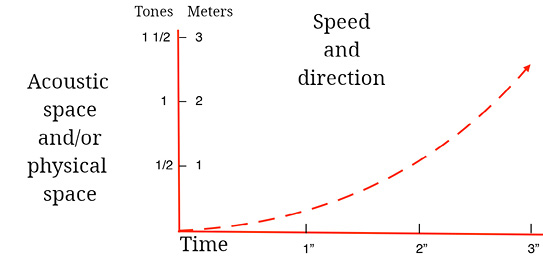
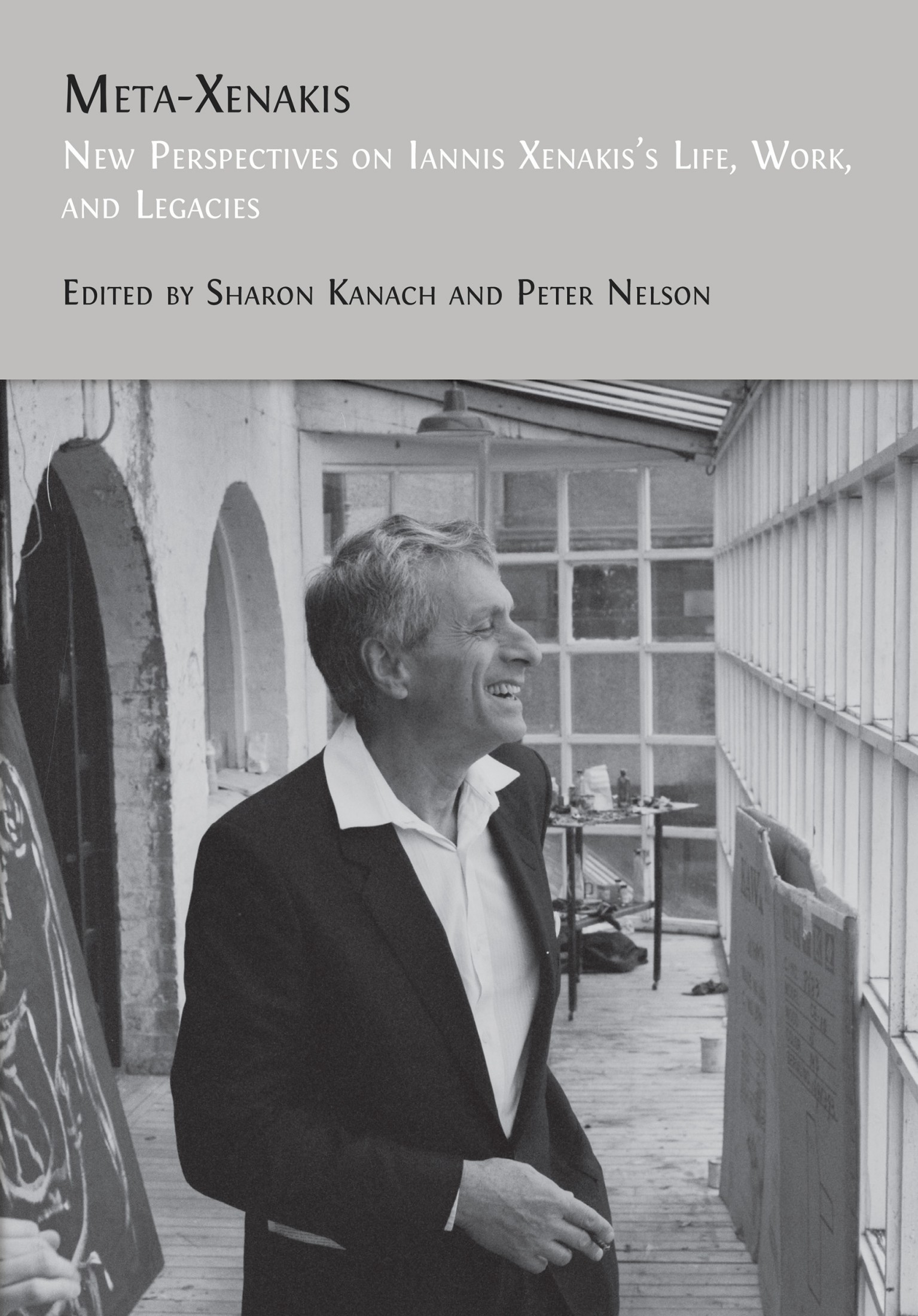
Fig. 13.2 Non-continuous displacement sound vectors. Impulses through fixed sources that divide the physical or acoustic space. Although the sources do not move, the synchronized impulses seem to travel through the physical or acoustic space with specific speed and direction. Figure created by author (2022).
Non-continuous displacement outlines a trajectory through fixed sources that divide the physical or acoustic spaces in a determined way. The sources do not move, but the synchronized impulses they produce with a determined speed give the impression of an impulse that is transmitted with a certain speed and direction, creating a sound vector.
Thus, any rhythmic-melodic sequence can be considered a sound vector in the acoustic space. These sequences are not perceived as isolated points, but as impulses with an identity, despite the constant fluctuation and the melodic leaps of some melodies—very wide, as in Anton Webern’s (1883–1945) Five Canons on Latin Texts, Op. 16, or very small, as Julián Carrillo’s (1875–1965) microtonal quarter-tone steps.
Fig. 13.3 Examples of extreme melodic trajectories: Anton Webern’s 5 Canons, Op. 16, No. I (1923–4), voice part, and Meditación, from Julián Carrillo’s 2 Bosquejos pour quatuor en quart de ton (1927), No. 1, violin I part in quarter tones (dates given are dates of composition).1 Figure created by author (2022).
In his text The Musical Timespace, Erik Christensen refers to the acoustical space when he writes “Melody is the spatial shape of music.”2 But the spatial shape can also be organized in physical space through a particular spatial distribution of fixed sources and the synchronization of the impulses they produce. The perception of continuity of the impulse depends on factors such as the distance between sources, the transition velocity from one source to another—a very important aspect that I will discuss below, the duration of each impulse produced, its dynamics and timbre, and the location of the listener, among others. Both spatial shapes, i.e., the melodies, and the synchronized impulse, are transmitted between discrete points in acoustic and physical spaces.
One of the clearest interfaces that shows the connection between physical space and acoustic space is the keyboard in instruments like the piano or the harpsichord. This interface is a mechanism that assigns a different pitch to every key. The harp is another instrument that beautifully shows this special distribution and its correspondence in the acoustic space. These instruments produce non-continuous displacement sound vectors that are transmitted among fixed sources in the acoustical and physical spaces with given speed and direction, although the trajectory they form does not travel through each and every point of the acoustic or the physical space.
To perceive the sound vectors produced by the harp or the piano in physical space, one must be close enough to the instrument to distinguish separately each point of sound production. If one is far enough away, the sounding board acts as a diffuser, and it becomes more difficult to distinguish each sound production point. In the marimba, that has an individual resonator for each key, sound vectors in physical space can be perceived even if one is not very close.
I find the glissando on the piano and the harp of special interest. It forms a sound vector in the physical and the acoustic spaces. Its great speed in the succession of sounds seems to cancel the distance between the strings, giving an impression of continuity in both spaces. Hence the name glissando (from French glisser, meaning slip or slide). What is really happening is that our ear cannot distinguish each separate event in time or in either space, and it groups everything as a sound mass with its own speed and direction. I will discuss this phenomenon below, where I analyze Persephassa (1969) by Iannis Xenakis.
I also find an analogy between sound vectors in space and light-series, dancing fountains, and lenticular paintings (Figure 13.4). In this case, paths formed by discontinuous elements can be perceived.
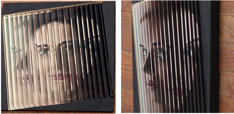
Fig. 13.4 Maria. Painting with lenticular effect by Lucía Andrade. © Lucía Andrade, reproduced with the artist’s permission.
From now on, I will use the term “sound vectors” to refer to non-continuous displacement sound vectors, unless otherwise specified.
Sound Vectors in Original Compositions
In 1993, during a presentation of Conlon Nancarrow’s (1912–97) studies by the kinetic sculptor and sound artist Trimpin (b. 1951), on a marimba keyboard, I could observe that the rhythmic-melodic impulses of Nancarrow’s canons for player piano, adapted for a sculpturally spatialized rearrangement of the keys of the marimba by Trimpin, moved with several velocities through space, and it occurred to me that it was possible to synchronize similar events with other performers.3 In 1998, I explored these possibilities with the first version of my piece for thirteen trombones Atecocoli (“seashell” in Nahuatl, a prehispanic language of Mexico). It was carried out in the courtyard corridors of the National School of Music, UNAM—today’s Music Faculty—during a homage to Nancarrow after his death. I chose thirteen trombones to recall thirteen seashells, whose sonority was typical of prehispanic cultures. At this time, I had no knowledge of the works Orbits (1979) for eighty trombones, organ, and sopranino voice by Henry Brant (1913–2008), or Trombonhenge (1980) for thirty trombones by Charles Hoag (1931–2018). Both compositions were designed to make use of the location of the trombones surrounding the audience. There are no sound vectors in these works because the group of musicians is not evenly distributed around the audience, and so do not produce the effect of continuous displacement of sound impulses.
In my opinion, this version of Atecocoli was a relative disaster given the difficulty of designing a score that allowed the performers to control the sound events. My purpose was not only to locate the performers in a specific space, but to map out sound trajectories with a certain speed and direction, which I now call sound vectors in physical space. For this I had to synchronize the sequence of events of each performer with great precision, which I solved with a multi-tempi MIDI sequence. To solve the problem of transmitting the audio signal with a pulse with a specific speed (that was independent of all the others) to each performer, being a considerable distance apart from the other performers, I needed very long cables to connect the MIDI modules with independent outputs for every channel, as shown in Figure 13.5.
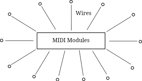
Fig. 13.5 Wiring from MIDI modules to thirteen points in a circle. Figure created by author (2022).
Another problem was to assemble, without a budget, thirteen trombone performers practically without any rehearsal. The participation was very enthusiastic, and the result showed me the potential of the system, although the desired result was not met.
As I already mentioned, making a useful score that allowed me to write clearly and with precision was one of the first problems I encountered. Figure 13.6 is a fragment of the score of this performance:
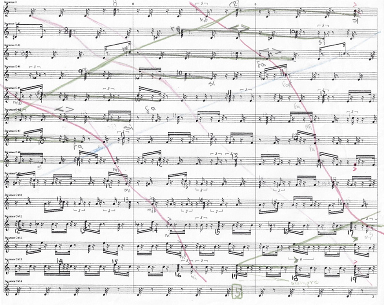
Fig. 13.6 Rodríguez Lara, guide notation for Atecocoli 1998.
This score is the conversion to notation of the MIDI events page. It was made in the Studio Vision sequencer. As can be observed, there is a lot of information concerning the pulses of each sequence—which is the graphic representation of the multi-tempi, but it hinders the visual organization of the score, even for something as elementary as writing the notes and duration of each event. I decided to trace with colored lines the trajectories chosen among all the pulses. This was a very rudimentary and inefficient technique, but it worked nonetheless and led me to the next step.
In the year 2000 I had the opportunity to explore the techniques required to achieve a score format that would allow for greater control of the notational elements: pitches, durations, dynamics, accentuation… practically every element of a “normal” score. With a series of strategies, I achieved a score format that graphically reflected the sequences of sound events in time. The first step in this process was the temporal organization of the sound events while this sequence of events is also planned as trajectories of displacement in space through the fixed sources.
For this new version, Atecocoli 2000, I could edit the sequence of events from Studio Vision to Finale, and in this score editor it was easier to remove all the elements that were not essential without losing the graphic placement of each event in the score.
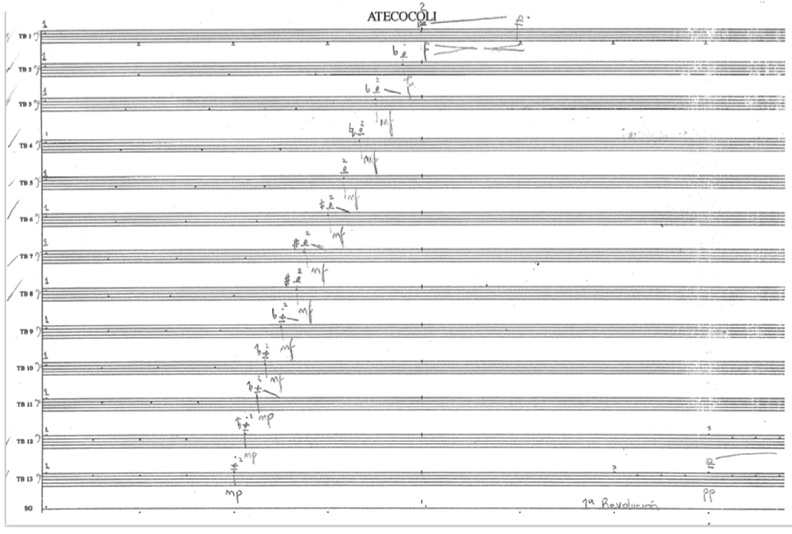
Fig. 13.7 Rodríguez Lara, score of Atecocoli 2000.
Techniques for Synchronizing Sound Vectors in Physical Space
For Atecocoli 2000 I used three synchronization techniques which I explain below.
Multi-tempi
The multi-tempi that I had explored in Atecocoli 1998 seemed to me like a relatively rigid grid to organize the pulses if followed for a certain time. I therefore used it only in small fragments, one of which is shown in Figure 13.8.
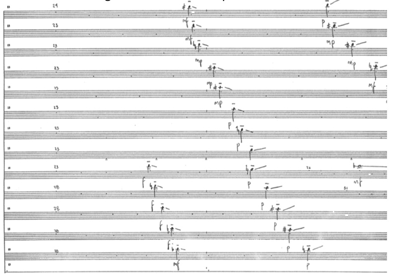
Fig. 13.8 Rodríguez Lara, Atecocoli 1998. Fragment in multi-tempi: each point of the score corresponds to a sound signal and is distributed independently on each channel. In total, there are thirteen simultaneous channels.
Anacruses
This is another very efficient synchronization technique. It consists of leaving each performer’s track unpulsed until a four-pulse anacrusis indicates, both on the performer’s particella and on the pulse recording, the time at which a particular event is to be played. This saves performers from having to count a sometimes-considerable number of silent beats before playing the next event, and allows greater flexibility in the placement of events not predetermined by a multi-tempi sequence:
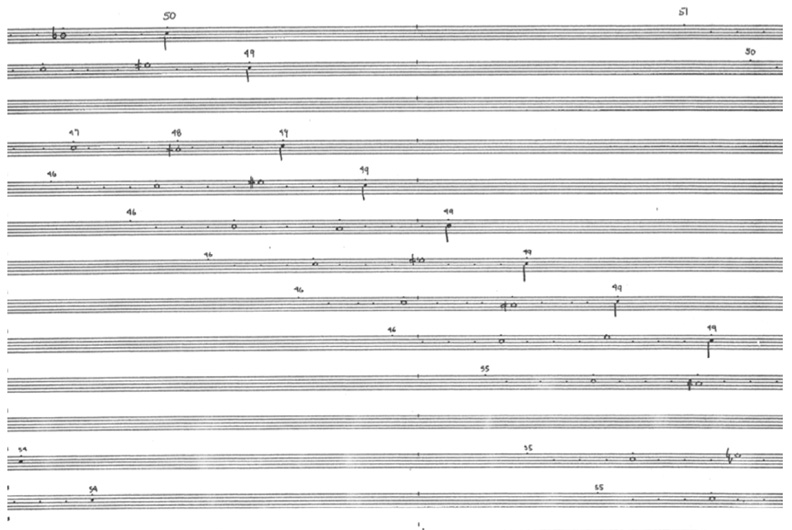
Fig. 13.9 Rodríguez Lara, Atecocoli 2000. Anacruses technique. Note that only when a performer is going to play a sound event, he or she prepares with a four-pulse anacrusis. There is silence from one anacrusis to the next.
Fine Phase Shift
Finally, another synchronization technique was the fine phase shifting of the same speed sequence. Towards the end of this version of Atecocoli, as a dense section, I used this technique. The offset shown is 1/13th of a second:
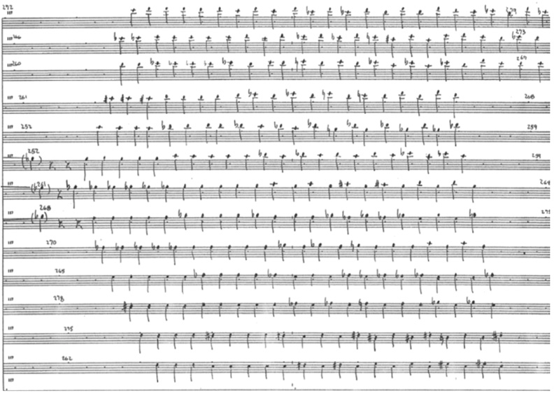
Fig. 13.10 Rodríguez Lara, Atecocoli 2000. Fine phase shift technique: a single constant speed sequence is shifted by 1/13th of a second.
Another piece composed in the same year and with similar techniques is Saxteto for saxophone sextet. The beginning is shown in Figure 13.11 below:
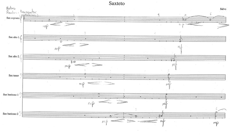
Fig. 13.11 Rodríguez Lara, Saxteto for saxophone sextet (fragment).
With these pieces, I was able to explore the behavior of more defined trajectories than in Atecocoli 1998. I believe the trajectory of sound vectors in physical space can be modeled by exploring their expressive possibilities more deeply towards a variety and a quality somewhat similar to the rhythmic-melodic and polyphonic elaboration carried out by composers of very different periods and styles, and interacting simultaneously with all the other factors of production of the sound event.
Other Compositional Possibilities with the Sound Vector Technique in Physical Space
Three possibilities that I find interesting to explore with this technique are the following: modeling of resonances, which reconstructs echoes of specific physical spaces; the atomization of texts, which is applicable to poetry texts or vocal sonorities; and the projection in physical space of sound vectors with the temporal proportions of harmonic sounds.
Modeling of Resonances
Using the technique of sound vectors in physical space, it is possible to configure, to a certain extent, the resonance patterns (behavior of the echoes) of a sound in a particular space from the articulation pattern of the sound and its decay time. This resonance is characteristic of certain locations, and can be projected into another space (container space) with its own resonance patterns reconstructed through the sound vectors in the physical space. The result of the interaction between the resonance of the reconstructed space and the resonance of the container space could be considered a virtual multi-space, as if the container space contained, at the same time, the acoustic characteristics of other spaces.
For now, I will only discuss the configuration of resonant echoes, which have a characteristic temporal pattern of articulation and a characteristic decrescendo. It is also possible to keep the echoes at a single point (with one source) or to shift the emission of the echoes, as if the echoes were “bouncing” in space or moving linearly in various directions. Echoes can be treated as sound vectors in physical space. It is even possible to model echoes in the opposite direction: anti-echoes whose resonance is presented in crescendo and ends with the “real” sound, although this is a very artificial contour.
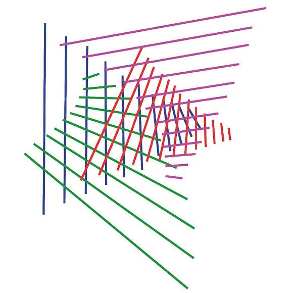
Fig. 13.12 Graphic representation of a virtual multi-space. Figure created by author (2022).
Atomization of Texts and Sound Poetry
In the genre of sound poetry, it is possible to project texts on a given space with the technique I call “atomization.” This technique consists of assigning a word, a syllable, or even a letter of a word, whether vowel or consonant, to different sources-interpreters placed in different spots. In the sonority of the vowels, as in traditional music, it is possible to assign notes, durations, intensities, and some variations of the timbre. It is also possible to configure melismas as sound vectors in physical space.
In order to accomplish this, I classify the sonority of the usual consonants in Mexican Spanish by their articulation, their capacity to extend their duration, and their sonorous quality as follows: 1) short, explosive consonants that cannot extend their duration are [c (k, q)], [p], and [t]; 2) friction consonants, with air noise that can extend their duration are [f], [j (x)], and [s (z)]; and finally, 3) the consonants that can extend their duration are [b (w)], [d], [g], [l], [ll], [y], [m], [n], [ñ], and [r] (frullato). In consonants that can extend their duration there are a considerable number of timbre and color possibilities when varying the frequency.
Atomization is then the process of fragmentation of the sonority of a word or phoneme, according to these principles, and modeled as described above so as to enrich its expressive character.
Projection in Physical Space of Sound Vectors with Temporal Proportions of Harmonic Sounds
In his famous text New Musical Resources, 4 Henry Cowell (1897–1965) proposes the use of rhythmic values derived from the proportions of harmonic sounds, so that one can hear, as durations in time, values in the same proportions that present certain harmonics in the frequencies of the sound:
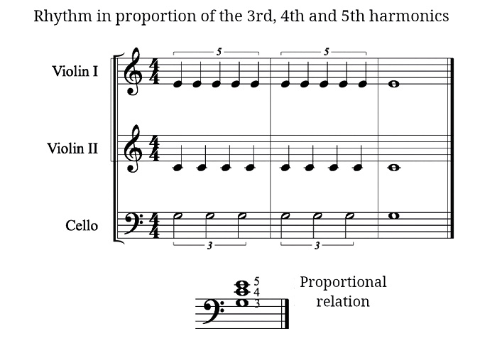
Fig. 13.13 Relationship based on Henry Cowell’s proposal between rations of natural harmonics and rhythmic durations. Figure created by author (2022).
Harmonics are phenomena that occur naturally in the acoustic space, and they have a very precise proportional order. And, as Cowell proposed, using a projection of the proportions in the frequency of the harmonics onto the temporal durations of rhythmic-melodic sequences, sound vectors can also be projected onto physical space based on the same proportions:
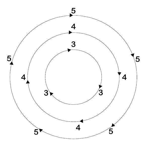
Fig. 13.14 Distribution of sound vectors in physical space: circular trajectories with the same proportion of the 3rd, 4th, and 5th harmonics. Figure created by author (2022).
Examples of sound vectors over wide physical spaces can be found among the following compositions, all from the second half of the twentieth century: Karlheinz Stockhausen’s (1928–2007) Gruppen (1955–7); Xenakis’s Terretektorh (1965–6), Nomos Gamma (1967–8), and Persephassa (1969); Julio Estrada’s (b. 1943) Canto Naciente and Eolo’oolin (1981); Llorenç Barber’s (b. 1948) Vaniloquio Campanero (1993); and Saxteto and Atecocoli (2000), aforementioned compositions of my own.
Displacement of Events between Time and Physical Space
Now we will explore the difference between speed considered as the number of events in time, and the speed of the displacement in physical space of an event, a difference that is more evident if that event is an articulated sound. Consider a short event that does not move in acoustic space and occurs every second, for example, a clap. Eight performers are placed in space in a defined path, either curved or straight. If an event is assigned to each performer consecutively, then a displacement in time equivalent to the movement in physical space is heard, as shown in Figure 13.15.
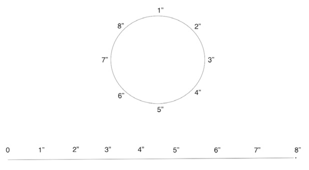
Fig. 13.15 Example of movement in time and in physical space. This event moves in different trajectories in physical space through time in a constant pulse of one second. Figure created by author (2022).
Now, we will think of a faster repetition of the event, such as a tremolo on a percussion instrument, and let us consider each stroke of the tremolo as an event. If a certain number of repetitions of the event are assigned to each performer, the speed with which the event moves in physical space will be slower that the speed regarded as the number of events per time unit. It is even possible to create a counterpoint between these factors: a sound event that presents an acceleration in time and a deceleration in physical space, or that maintains the speed of the event in time and accelerates its displacement in physical space, as we will see below in Persephassa by Xenakis. This is only one among many other possibilities of interaction.
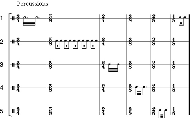
Fig. 13.16 Example of a tremolo moving in physical space accelerating between five performers. The duration of the notes of each performer is shortened and the spatial motion is accelerated, but the speed of the tremolo remains constant. Figure created by author (2022).
Persephassa
Xenakis’s Persephassa for six percussionists placed at homogeneous distances around the audience (Figure 13.17) features several passages that, in my opinion, would fall into this category; especially the final section of the piece which features a series of tremolos distributed among the instruments of the six percussionists in order to give the impression of accelerating rotations.
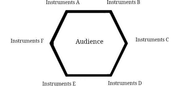
Fig. 13.17 Xenakis, Persephassa (1969): distribution of the performers around the audience.5 Figure created by author (2022).
For this analysis, as I already mentioned, it is necessary to consider that one sound event is one stroke that is part of the tremolo and not each notated value that may contain a certain number of repetitions for its duration. If the notation gradually shortens the duration of the notes played in the tremolo, or if the pulse is accelerated, an acceleration of the rotational movement of the impulses will be perceived, but the speed of the tremolo will remain constant. In other words, each event (tremolo) occurs at a constant speed in time and with a high value extending over the duration of each note; these notes will gradually shorten their duration and thus move more quickly in physical space.
As Maria Anna Harley describes it:
The climax of Persephassa (mm. 352–455) begins with a slowly rotating tremolo on the drums (four tom-toms and two snare drums) to which other timbrally distinct layers are gradually added, thus increasing the density of the texture […]. The superimposed cycles of rotations are performed on metal simantras (from m. 354), cymbals (from m. 357), Thai gongs (from m. 361), wooden simantras (from m. 369), tam-tams (from m. 381), and woodblocks (from m. 395). The seven layers alternate in direction and differ in their starting points.6
Simantras are metal or wooden instruments, ancient in origin, but designed in reconstruction by Xenakis. Harley also writes:
The seven layers of tremolos move 8 times faster at the end of their cycle of rotations than at the beginning, while the following solitary cycle of drum tremolos revolves 12 times faster than the same drums at the beginning. In Terretektorh, accelerations were constructed as segments of spirals; here, a large-scale temporal spiral is built from many individual ‘circles’ of increasing tempi.7
These cycles, which are distinguished by the timbre of each tremolo, are sound vectors: impulses with speed and direction, distributed in six zones of space. But again, the speed of each temporal event—each stroke of the tremolo—remains constant over time, while the displacement in physical space produced by the duration of the notes is shorter and shorter, and this is what causes an acceleration.
I also notice a very interesting effect on the physical space: due to the speed at which the notes move, it seems that there is less distance between the sources. In their spatial arrangement, the performers occupy what would correspond to a whole-tone scale in the acoustic space: six places dividing a circle of certain dimensions into homogenous distances. But the number of events per second gives the impression of greater proximity, as if there were a shorter space between them.
This phenomenon seems to me to be similar to a glissando on the piano or the harp (Figure 13.18). In this case, the impulse generated by pressing the keys, upwards or downwards, is so fast that the ear does not have time to process each sound produced individually and perceives a sound mass that moves with a certain speed and direction, as if the whole frequency field were being traversed in a continuous glissando. What actually happens is that it only travels through the white key scale or even the black key pentatonic scale with great speed. Again, the speed of succession of events gives the impression that the distance between sources, in acoustic and physical space, is shorter.
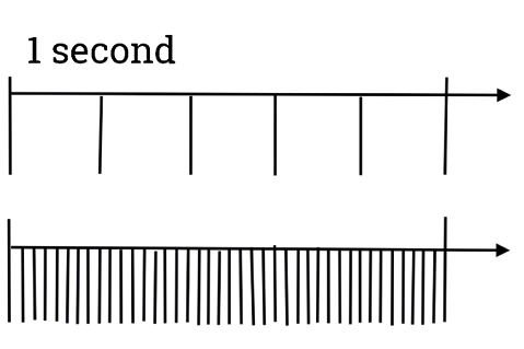
Fig. 13.18 Graphic representation of the effect of cancellation of the acoustic or physical space in a very fast presentation of events in one second. There is a tendency to perceive a certain continuity of the impulse. Figure created by author (2022).
Another very remarkable example of this phenomenon can be found in the final section of Nancarrow’s Etude 21, Canon X (1960), in which the transition of 110 events per second over the area of the strings of the player piano produces the impression of a turbulent, oscillatory cloud in physical space of the instrument. The intensity is increased by the number of attacks per second, and the sequence of pitches is also transformed into a timbre (in acoustic space). It is important to notice that in these cases, despite the speed, the Doppler effect does not occur because the sound sources themselves are not moving.
Conclusions
I consider rhythmic-melodic movement to be a sound vector in acoustic space, that is, a sound impulse with speed and direction. In acoustic instruments that are constructed with fixed sound producers, be they strings, wooden or metal keys, and ordered from the lowest to the highest pitch in a single direction, the rhythmic-melodic impulses will produce sound vectors in acoustic space and also in physical space, even if this space is reduced to the size of the instrument. With technological resources, it is possible to apply a similar projection of sound vectors, but over much larger and more varied physical spaces.
There are pieces by twentieth-century composers who have handled sound vectors in physical spaces of specific dimensions and conditions. Some of these vectors are carefully calculated, as in Stockhausen’s, Xenakis’s, and Estrada’s works, and in my own works. Other vectors have a margin of limited uncertainty, as in Barber’s works for city bell towers.
I consider the projection of sound vectors in a physical space as a certain extension of what occurs in the acoustic instruments here described. But, as Nancarrow achieved a control of very complex rhythmic events in his studies for player piano, many of them impossible for humans to execute directly, the techniques I propose allow for the management of temporal resources and their projection as sound vectors in physical space. These resources cannot be realized with other media, but they have a great expressive potential.
References
BLESSER, Barry and SALTER, Linda-Ruth (2007), Spaces Speak, Are You Listening?, Cambridge, Massachusetts, MIT Press, https://doi.org/10.7551/mitpress/6384.001.0001
CARRILLO, Julian (1982), Dos Bosquejos pour quatuor en quart de ton (JJ 09153), Paris, Editions Jobert.
CHRISTENSEN, Erik (1996), The Musical Timespace: A Theory of Music Listening, Aalborg, Denmark, Aalborg University Press.
COWELL, Henry (1930), New Musical Resources, Cambridge, United Kingdom, Cambridge University Press.
FELER, Coline (2016), “Karlheinz Stockhausen. Gruppen para tres orquestas” (14 July), Música en México, https://musicaenmexico.com.mx/karlheinz-stockhausen-gruppen-3-orquestas/
HARLEY, Maria Anna (1994), “Spatial Sound Movement in the Instrumental Music of Iannis Xenakis,” Journal of New Music Research, vol. 23, no. 3, p. 291–314.
ISCM (1993), Program of the festival Días de la Música: Ciudad de México (November 20–7), p. 165, https://iscm.org/wnmd/1993-mexico/
MORITZ, Albrecht (2005), Stockhausen. Gruppen (1955–1957), https://www.stockhausen-essays.org/gruppen.htm
WEBERN, Anton v. (1928), Fünf Canons, Op. 16 (score UE 9522), Vienna, Universal Edition.
1 Transcript of Webern, 1928, mm. 2–5 and of Carrillo, 1978, mm. 1–4.
2 Christensen, 1996, p. 98.
3 This was at the Conlon Nancarrow Exhibition in the Palacio de Bellas Artes, in Mexico City from 23–7 March 1993. See ISCM, 1993.
4 Cowell, 1930, p. 52.
5 Diagram based on Fig. 11 in Harley, 1994, p. 306.
6 Ibid, p. 307
7 Ibid., p. 307–8.