31. UPISketch: New Perspectives

Rodolphe Bourotte

When we consider the needs we may have in the field of electroacoustic music composition, a tool allowing a graphic representation of sound and musical phenomena may seem interesting to develop. UPISketch is one of these tools.1 This presentation will focus on describing the abundance of ideas that the development of such a tool can inspire. UPISketch is a subset of graphical score systems: it is positioned on the question of graphical representation of quantitative data. This is a particular posture, one that has its roots in the following statement:

Music notation is the representation of several physical values evolving over time. Since the nineteenth century, experimental physics has made much use of graphs and plots—visual representations to visualize experiments or observations. Interestingly, the notation of music is a reversed process compared to scientific graphs: instead of representing observed values, music notation describes, like a timed map, the physical state we seek to observe (with our ears) in our environment at successive moments.2

In this sense, it can update the breakthroughs that Xenakis made through his mathematical approach, by making them newly accessible via an intuitive graphic interface. Possibilities, in the process of implementation, will be evoked, both on the graphical aspect and for sound synthesis. The legacy of Xenakis’s research on sieves and probabilities is inescapable, and it is possible to imagine an extension of it in the graphical domain with UPISketch, in a junction that had never been realized with UPIC (Unité Polyagogique Informatique du CEMAMu (Centre d’Études de Mathématique et Automatique Musicales)).

UPISketch is a sound composition tool, which was developed by Centre Iannis Xenakis (CIX) in 2018 in cooperation with the European University of Cyprus within the framework of the Creative Europe Interfaces Network. Its development was part of the Interfaces action “Urban Music Boxes and Troubadours.”3 The impetus for the project came from the fact that, more than ten years after UPIX (UPIC software version) development was halted, no software had all the following characteristics:

• An intuitive interface that makes it possible to quickly produce a composition, even without musical or computer experience.
• A short reaction time between the user’s gesture and the resulting sound or image.
• Each drawn curve has an internal representation, and its parameters can be individually determined.
• Drawings can be extremely precise.
• Drawing and sound synthesis tools are integrated (no external software dependencies required).
• The basic physical values are frequency and intensity.

The table below illustrates the differences between some possible UPIC epigones:

Table 31.1 Table of UPIC epigones.

Since the Interfaces Creative Europe project’s completion in 2020, we have had the possibility to further develop UPISketch, so it can be used not only on tablets, but also on desktop computers: using Windows, Mac, and Linux operating systems, the latter since 2022 thanks to the contribution of Rodney DuPlessis, then a PhD candidate in composition at UCSB.4

Xenakis’s centennial in 2022 and the Meta-Xenakis consortium offered the opportunity to launch the first International UPISketch Composition Competition.5 The internationality of submissions was impressive: participants came from eight countries and four continents. This event allowed us to receive a lot of documented material on the composition process using UPISketch, and also a good amount of user feedback, both of which are helpful in guiding the next steps of development as well.

A few words should be said about the first method of synthesis that was implemented in UPISketch. There was the wish to take advantage of the richness inherent in already existing sounds, whether they come from acoustic or synthesized instruments. This decision triggered the interest for providing a library of default sounds.6 With UPIC, one could load a waveform, representing a tiny portion of the information that a natural sound contains. All UPIC users experienced this limitation. Therefore, we extended this to the duration of a note, or even a phrase of several seconds, which allow access to other aspects of timbre or timbral evolution over a longer term.

Figure 31.1 shows the principle of the synthesis: we choose existing periods of a sound, and rearrange them by resampling, removing, or duplicating some of them when necessary.

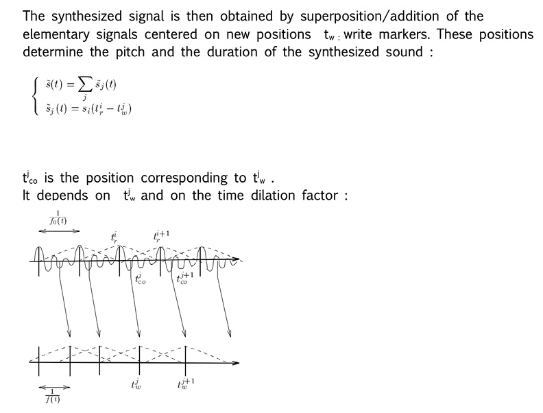
Fig. 31.1 Excerpt from the first UPISketch milestone specifications © CIX 2017, reprinted with permission.

But there is a drawback in this principle: this technique introduces the necessity to analyze the fundamental pitch of the original sound. This is an imperative step in order to recreate a sound at a different pitch from the original, when recreating it in the time domain. Such an analysis can be made, for example, with the program Tony.7 From there we dispose of a list of pitches versus time. Willing to impose an absolute pitch to this sound implies that we calculate, for each analyzed pitch, the transposition to apply in order to obtain the desired pitch.

Table 31.2 Transposition inferred from desired pitch and actual analyzed pitch.

However, as the first UPICian postulate was to propose an efficient, fast, and easy (intuitive) interface that even children could use, it was necessary to call upon an automatic analysis of this fundamental pitch. Being automatic makes it fallible, hence in turn it can sometimes produce undesirable—or interesting—artifacts…

Not only for historical reasons, but also to be open to new types of synthesis allowing more reliable and precisely reproducible results, in the version 3 of UPISketch, released in 2022, we proposed pure oscillators. Using the default definitions entails selecting a default synth prior to drawing, and then verifying by visualization what it has done:

Media 31.1 Output sound exported from UPISketch, viewed in Audacity.
https://hdl.handle.net/20.500.12434/8410c834

To go further we can also define a waveform by using a mathematical expression. This has been made possible by the exprtk library by Arash Partow.8 Some examples of the syntax in this library are presented below:

(00) (y + x / y) * (x - y / x)

(01) (x^2 / sin(2 * pi / y)) - x / 2

(02) sqrt(1 - (x^2))

(03) 1 - sin(2 * x) + cos(pi / y)

(04) a * exp(2 * t) + c

(05) if(((x + 2) == 3) and ((y + 5) <= 9),1 + w, 2 / z)

(06) (avg(x,y) <= x + y ? x - y : x * y) + 2 * pi / x

(07) z := x + sin(2 * pi / y)

(08) u := 2 * (pi * z) / (w := x + cos(y / pi))

(09) clamp(-1,sin(2 * pi * x) + cos(y / 2 * pi),+1)

(10) inrange(-2,m,+2) == if(({-2 <= m} and [m <= +2]),1,0)

(11) (2sin(x)cos(2y)7 + 1) == (2 * sin(x) * cos(2*y) * 7 + 1)

(12) (x ilike ‘s*ri?g’) and [y < (3 z^7 + w)]

Code 31.1

This is a first implementation, and as specified in the UPISketch documentation, the modification of such definitions is likely reserved for experienced users.9 However, in an upcoming version, formulas will be much easier to use and saved with the UPISketch project (.upixml). Math expressions will be entered this way:

Media 31.2 Tweaking the waveform definition for math expression synthesis.
https://hdl.handle.net/20.500.12434/b537144c

By assigning this edited expression, 2 * sqrt (1 - (x / (2 * pi)) ^ 2) - 1, to a gesture, we obtain the following output: a quarter of a circle repeated on each period. The variable x stands for the angle between 0 and 2π, which is updated at each new sample, according to the drawn pitch.

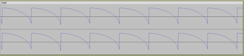
Fig. 31.2 Resulting waveform from math expression: 2 * sqrt (1 - (x / (2 * pi)) ^ 2) - 1. Figure created by author (2022).

Seen in a xenakian context, splines represent a very interesting topic. The Génération Dynamique Stochastique (GENDYN)10 method invented by Xenakis is well known, and uses breakpoint functions to define a single period of sound, as well as functions which control points that are modified stochastically at each period:

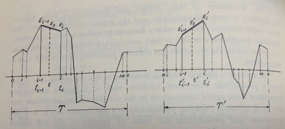
Fig. 31.3 GENDYN graphic description.11 © Pendragon Press (1992), reprinted with permission.

There have been several modifications to this first proposition, notably using splines, under the supposition that this mathematical object may represent the way sound pressure is propagated in the air in a more natural fashion by any kind of acoustic instrument. Obviously, we can object that this could be a step backwards on the search for unearthly sounds. However, maybe the straight lines chosen in 1991 were, in fact, chosen because of some computer limitations? In any case, here are some examples:

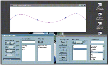
Fig. 31.4 SplineSynth © Nick Collins (1999), reprinted with permission.

Media 31.3 Spline waveform modulation. © The author (2017).
https://hdl.handle.net/20.500.12434/8432bfdf

Now, with the participation of Matt Klassen, we are working on implementing an original form of synthesis, based on a simplified vector representation of audio.12

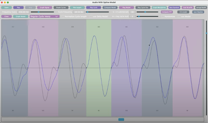
Fig. 31.5 Audio spline interpolation demo video screenshot.13 © Matt Klassen (2022), reprinted with permission.

Several innovative aspects in Klassen’s work can be mentioned:

• He starts from existing sounds and makes a vector interpolation from splines.
• He introduces the notion of keycycles, the equivalent of keyframes in animation software.
• This technique allows a high level of information compression: if you want to mix several sources together, rather than calculating the temporal interpolations between keycycles for each of the voices and then adding these voices together, one only needs to interpolate first the keycycles themselves, and then perform a single temporal interpolation.

“Very Free but Accurate”14

Now, I would like to relate some more personal thoughts, related to my musical practice.

Thinking about the question of the aleatory and the continuous, this indication at the beginning of one of Paul Méfano’s (1937–2020) scores comes to mind:

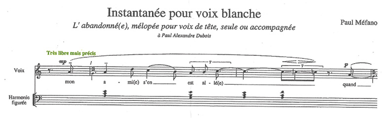
Fig. 31.6 Excerpt from L’abandonné(e), score by Paul Méfano © BabelScores (2000), reprinted with permission.

Not only the aleatory in music can be a conceptual tool in composition, it also can raise a number of issues regarding notation and interpretation. The history of written music shows a variety of ways to address accuracy. Even if centers of interest may change, in general, there is a large amount of information to be dealt with by the interpreter. The following score, for example, focuses rather on proposing to get into a certain state of mind. The musician can also be asked to raise his/her awareness and self-relation to the sound and the environment, etc.

for at least the next half hour.15

I will not argue here about the value of different approaches concerning which musical information should be fixed by the composer. The very thing I am interested in is how to create complexity in a simple way. For example, the identity of a piece does not necessarily depend on the exact predetermination of the sound events that compose it. A musical piece can be seen as a succession of statistical characteristics. This is where Xenakis intervened. In pieces like Pithoprakta (1955–6) or Metastasis (1953–4), changing one sound here or there in the final score would be harmless. A real change would rather come from a modification of the overall statistical tendencies. Indeed, we can be tempted to organize things on a different level:

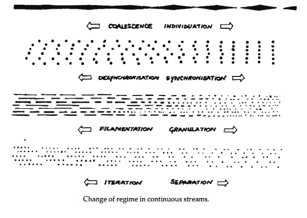
Fig. 31.7 Some musical production typologies, as illustrated by Trevor Wishart.16 © Trevor Wishart and Simon Emmerson (1996), reprinted with permission.

This schema advocates again for a global control rather than defining each and every single event. Nature itself is “very free but accurate.” The following statement may sound especially obvious nowadays, with the advent of artificial intelligence (AI) image generators, but it is worth keeping our context in mind: the image below could be very different in the details of its geometry, but we would nevertheless feel the same looking at it, sensing its overall aspect.

Fig. 31.8 Photograph of a shore in Brittany, by the author (2022).

I have explored two ways of managing these so-called global variations for populations of sounds:

• One, in an analogic way (score on paper), by adding symbols expressing choices or limits within which the values must be contained, or by indicating mean values with an amount of possible deviation. This is no exclusive novelty, yet here is how I gave indications of tendencies within my piece Interrupted Exceptions (2005):

Fig. 31.9 Excerpt from Interrupted Exceptions, score by the author (2005).

• The other way, digitally, with a real-time display device, that would start work from the same paradigms: I call this system Comma.17 Media 31.4 shows what it looked like some years ago.

Media 31.4 Comma (2004), Max/MSP and cathodic screens.
https://hdl.handle.net/20.500.12434/56bfb6e1

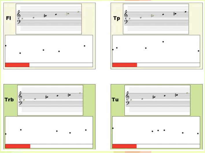
Fig. 31.10 Comma, screenshot (2004). Figure created by author.

The particularity in both cases (the analogic case of Interrupted Exceptions and the digital case of Comma), is that the composition consists of describing in real time the evolution of random parameters, such as density, rhythmic regularity, dynamic agitation.

Below is an example of a meta-score:

Fig. 31.11 Comma, hand-drawn meta-score (2018). Figure created by author.

…with, in Figure 31.12 below, the way it has been entered in Max/MSP, so that it would send information to my other software (CommaTransmitter/CommaReceiver) via Open Sound Control (OSC):

Fig. 31.12 Comma meta-score as translated into 2D curves in Max/MSP (2018). Figure created by author.

This meta-score feeds the CommaTransmitter, which in turn sends the appropriate instructions to the CommaReceiver owned by each instrumentalist. A second phase in the development of this tool occurred in 2018, thanks to a residency at the European University of Cyprus in the framework of the same Creative Europe project Interfaces, at the end of which we set up a group of instrumentalists to play around with the new version, running under OSX and iOS.18

There is a difference though between Interrupted Exceptions and Comma. In the former, the performer has to interpret symbols to generate the events; while in the latter, events are directly read, as they are already generated by the CommaTransmitter application.

Information Density

There is another challenge regarding the control of multiplicity. We have shown that in the history of Western written music there is a growing interest in multiple characteristics of sounds. This has resulted in a global increase in the quantity of described musical information: pitch, tempo, dynamics, timbre… Furthermore, it is interesting to note that be it in the case of a score with only pitches or of an ultra-detailed score, there is always additional information that escapes notation. In both cases, the composer expects something “very free but accurate” but deals with the human factor of the performance in a different way. (See Fig. 31.13.)

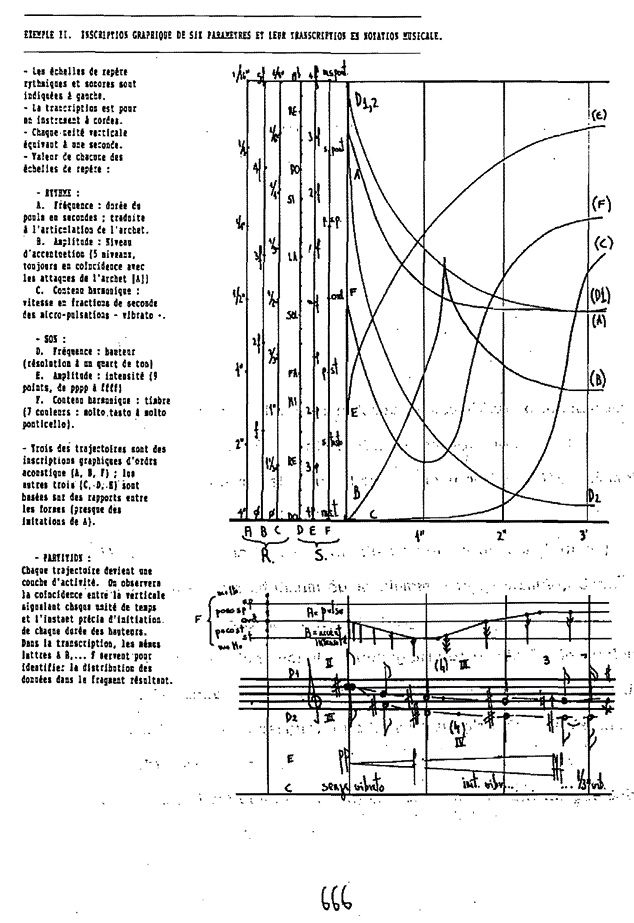
Fig. 31.13 Julio Estrada, Théorie de la Composition (II), p. 666.19 © Julio Estrada (1994), reprinted with permission.

This evolving musical mindset has induced the need to find a way to manage all this information without being overwhelmed; also in electroacoustic music where, a priori there is no limitation of the number of parameters. For instance, how would we control—in an intelligent manner—an audio plugin when the plugin covers 165 parameters?!

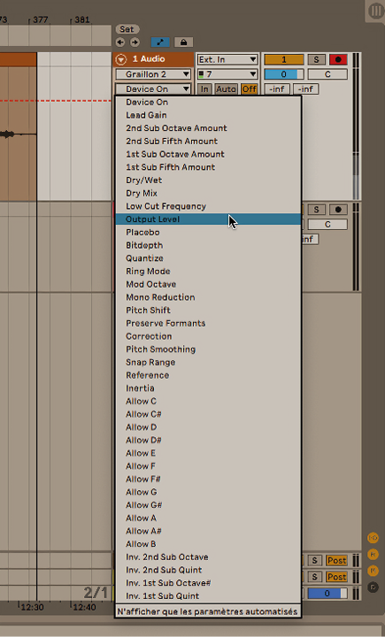
Fig. 31.14 List of parameters held by an example plugin (2022). Figure created by author.

The answer resides in creating meta-parameters that define sound objects more globally. A sound would then be defined by the position of a meta-parameter in a multidimensional space. There is still a lot of ongoing research in this domain, since the representation of such a space, either in 2D or 3D, is quite insufficient. Indeed, “small-D” implies the superposition of several curves and forbidden trajectories. To understand this, it suffices to try to describe graphically, in two dimensions, the position of a point in a 2D space versus time, which is the basic pitfall for graphically controlled ambisonic automation. To date, there is no clear-cut direction of work on UPISketch regarding this question.

UPIC-GENDYN, or UPISketch-Comma Unification

From the reflections above, we may infer the following: we are interested in unifying the two very different concepts residing respectively in UPIC and GENDYN. This is not a new concern as it has been evoked in the past by Peter Hoffmann:

Indeed, it could have been interesting to integrate GENDYN synthesis within UPIC. Thoughts have been given to this possibility (personal communication by Jean-Michel Razcinsky of CEMAMu in 1996). It is interesting to compare the UPIC system with the GENDYN program. They are in many aspects complementary, and it seems as if one concept compensates for the shortcomings of the other.20

This implies providing composers with a graphical editor of musical data in the form of drawn curves. But these curves would gain a special flavor: they would handle not only completely determined phenomena as is the case with UPISketch and UPIC, but also random ones, as with GENDYN and Comma.

It is also possible that UPISketch becomes an interface to control the Comma system. This would be a much simpler interface to use than the one created with Max/MSP. It would also allow a homogenization for access to both the production of music notation in real time, and the production of probabilistic sound events from the internal synthesis engine of UPISketch.

But, as it can also be good to get some perspective when examining an idea, I am also interested in comparing computer/no computer experiments. Such experiments will take place in 2024, thanks to the project tekhnē funded by the European Union in collaboration with the GMEA.21 Media 31.5 represents a start of an implementation, to get a feel of how this could work in UPISketch:

Media 31.5 A coded draft for a UPISketch probability drawing, using a pressure-sensitive device (drawing tablet and pen).
https://hdl.handle.net/20.500.12434/e19599e1

Interestingly, this approach may look like a representation of the wave function, the famous mathematical object used in quantum physics:

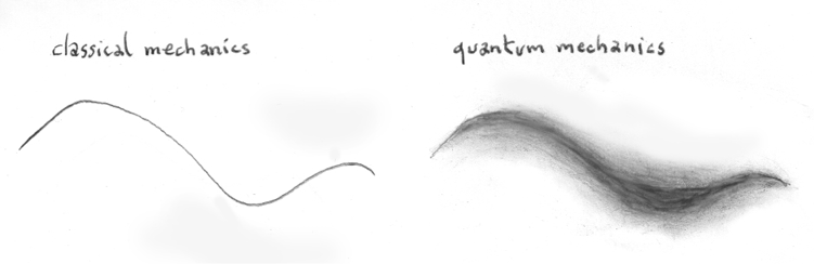
Fig. 31.15 A trajectory in classical mechanics, versus quantum mechanics (2022). Figure created by author.

Conclusion

Xenakis brought to musical creation more than his own music and more than formulas; he also awakened a state of mind and theoretical ferments which can only lead us to enrichment, both by the development of science, of techniques, and of our culture.

References

BOUROTTE, Rodolphe (2020), “Probabilities, Drawing, and Sound Synthesis: The Missing Link,” in Peter Weibel, Ludger Brümmer, and Sharon E Kanach (eds.), From Xenakis’s UPIC to Graphic Notation Today. Zentrum für Kunst und Medientechnologie Karlsruhe and Centre Iannis Xenakis. Berlin: Hatje Cantz, p. 291–306, https://zkm.de/de/from-xenakiss-upic-to-graphic-notation-today

BOUROTTE, Rodolphe and KANACH, Sharon (2019), “UPISketch: The UPIC Idea and Its Current Applications for Initiating New Audiences to Music,” Organised Sound, vol. 24, no. 3, 252–60, https://doi.org/10.1017/S1355771819000323

DELHAYE, Cyrille and BOUROTTE, Rodolphe (2013), “Learn to Think for Yourself: Impelled by UPIC to Open New Ways of Composing,” Organised Sound, vol. 18, no. 2, p. 134–45, https://doi.org/10.1017/S1355771813000058

ESTRADA, Julio (1994), “Theorie de la Composition: Discontinuum - Continuum. (Une Theorie du Potentiel Intervallique dans les Echelles Temperées et Une Methodologie d’Inscription Graphique et de Transcription de Parametres Rythmico-Sonores. Quelques Applications à l’Analyse et à la Composition Musicale,” doctoral dissertation, Université Marc Bloch (Strasbourg), p. 666, https://www.academia.edu/8455628/JULIO_ESTRADA_TH%C3%89ORIE_DE_LA_COMPOSITION_I_

HOFFMANN, Peter (2009), Music Out of Nothing? A Rigorous Approach to Algorithmic Composition by Iannis Xenakis, Berlin, Technische Universität Berlin Fakultät I - Geisteswissenschaften. Fakultät I - Geisteswissenschaften -ohne Zuordnung zu einem Institut. https://monoskop.org/images/3/38/Hoffmann_Peter_Music_Out_of_Nothing_A_Rigorous_Approach_to_Algorithmic_Composition_by_Iannis_Xenakis_2009.pdf

OLIVEROS, Pauline (2013), Anthology of Text Scores, Kingston, New York , Deep Listening Publications.

WISHART, Trevor (1996), On Sonic Art, London, Harwood Academic Publishers.

XENAKIS, Iannis (1992), Formalized Music: Thought and Mathematics in Music, additional material compiled and edited by Sharon Kanach (rev. ed.), Stuyvesant, New York, Pendragon.