6. Iannis Xenakis’s Free Stochastic Music Program as an Aid to Analysis

Ronald Squibbs

Introduction

In this chapter, I aim to do the following: firstly, to introduce Iannis Xenakis’s Free Stochastic Music program (both its history, and what it does); secondly, to explain how the code for the program became available to the general public; thirdly, to discuss the challenges involved in, and opportunities for, running the program today; fourthly, to present a sample of music composed based on a recent run of the program; fifthly, to examine a movement from Xenakis’s Atrées (1960), informed by practical experience with the program; and sixthly, to consider possible directions for future research on the program and on the works Xenakis composed with it.

The Free Stochastic Music Program

Xenakis’s program, Free Stochastic Music, was a computerized implementation of probability-based compositional procedures he had previously calculated by hand in the composition of works such as Achorripsis for chamber orchestra (1956–7) and in portions of Pithoprakta for orchestra (1955–6). The computer program allowed for a more thorough implementation of his ideas than had been possible previously. It was used in the creation of five works, generated between the years 1956 and 1962: ST/48, 1-240162 for orchestra, ST/10, 1-080262 for chamber ensemble, ST/4, 1-080262 for string quartet, Morsima-Amorsima (ST/4, 2-030762) for piano, violin, cello, and bass, and Atrées (ST/10, 3-060962) for chamber ensemble. The titles of these works indicate that they were composed using data generated by the stochastic program (“ST”) and the dates on which the data was generated by the Free Stochastic Music program. For ST/48, for example, the sequence of numbers “1-240162” indicates that the work was based on the first set of data generated on 24 January 1962. The sequences of integers in the titles of the works as a group show that the data for them was generated between January and September of 1962, with Atrées being the last work in the series. The earlier date in the range 1956–62 that applies to all five works indicates the year in which the planning for the project was begun.

The Free Stochastic Music program produces numerically encoded notations for sections of music which, within the program, are termed “sequences.” In finished compositions, the sequences may follow one another in order or the composer may choose to select from among them, reorder them, or combine them by presenting their contents simultaneously. The length of the sequence and the number of sounds the sections will contain are calculated first, with the specific properties of the sounds to be filled in afterward. The number of sounds per second, which Xenakis terms “density,” provides a quantitative measure of the texture in a sequence.

Next, the instrumentation of the sequence is determined. Within the ensemble defined for a specific composition, the instrumentation varies as a function of the sequence’s density. Controls are implemented so that the density (and therefore the instrumentation) varies gradually from sequence to sequence. This regulation of the changes in density represents a difference from the approach taken in the hand-calculated Achorripsis, for example, in which the changes in textural density were sometimes quite sharp. Sudden changes in density can add drama to a composition and can also help to delineate a work’s form as it unfolds in time. Gradual transitions in density can help the sequences blend into one another—if the order of the calculated sequences is maintained—but they can also have the effect of limiting opportunities for structural drama.

An additional six functions determine the qualities of an individual note: firstly, the time at which it begins; secondly, the instrument on which it is played; thirdly, its pitch if it is performed on a pitched instrument; fourthly, the characteristics of the glissando if it is performed on an instrument producing glissandi; fifthly, the duration of the sound; and sixthly, the dynamics of the note, which may be steady or changing.

The Free Stochastic Music program was run at IBM France on an IBM 7090 mainframe. The IBM 7090 was a multi-million-dollar, state-of-the-art computer system that was produced between 1959 and 1969. A description from an IBM technical fact sheet from 1960 reads, in part: “As a scientific computing system, the 7090 will greatly speed the design of missiles, jet engines, nuclear reactors and supersonic aircraft.”1 Xenakis’s use of this computer for the purposes of aesthetic creation represents a notable peacetime, non-commercial application of the computer system’s potential, providing a momentary respite to its normative military, aeronautic, and aerospace applications.

Documentation

Xenakis published the code for the Free Stochastic Music program, either in part or in full, several times during the 1960s and 1970s. Publication began in the French edition of his major treatise, Musiques formelles, in 1963.2 This was followed by the translation of the chapter on Free Stochastic Music from that book into German and English in the Swiss periodical Gravesaner Blätter (Gravesano Review) in 1965.3 The most complete publication occurred in the first English edition of Formalized Music in 1971 and was reprinted in the second edition of 1992.4 Between the publications of the 1960s and the later ones, the program had been updated from FORTRAN II to FORTRAN IV. Fortunately for current users of Fortran, the architecture of FORTRAN IV remained essentially intact in the next major update, FORTRAN 77, which runs on most modern Fortran compilers. The remainder of this discussion is based on the FORTRAN IV version of the program.5

The code alone is insufficient for interpreting the program’s output. To this end, Xenakis provided figures regarding essential details of instrumentation, dynamics, and texture. The most complete set of these figures is found in Formalized Music, which will be the source referenced here. Additionally, it is important to point out that most of the figures as well as all of the input data provided in Formalized Music refer specifically to Atrées, which will therefore be the only stochastic work discussed here.

Free Stochastic Music relies upon a precise classification of timbres and the instruments that produce them. Figure 6.1 shows a portion of the list of timbres and instruments for Atrées.6 The timbres are organized into classes, the first five of which are shown in the figure. To the right of the class numbers, the timbre classes are named, followed by the instruments that are used to produce those timbres and the numbers of the instruments within the timbre classes. It is important to note that an instrument may appear in more than one timbre class. For example, in addition to the glissando timbre class shown in the figure, the violin also appears in the following classes not shown in the figure: tremolo, plucked strings, struck strings (col legno), and bowed strings. To manage the multiple classifications of some instruments, the program identifies each sound source both by its timbre class and by the instrument producing that timbre.

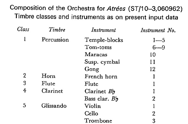
Fig. 6.1 Timbre classes in Atrées (excerpt) © Pendragon Press 1992, reprinted with permission.

The list of timbre classes in Figure 6.1 may imply that instruments are chosen freely from within their respective timbre classes. The choice of instruments, however, is constrained by the program according to probabilities that were predetermined by Xenakis and encoded in the program’s input data. An excerpt from the program’s output, shown in Figure 6.2, provides some information about the instruments in timbre classes 4 and 5, representing clarinet and glissando sounds. In the figure, the labels “HAMIN,” “HAMAX” etc. indicate minimum and maximum pitches (hauteurs in French).7 The reference pitch, 0, is equivalent to lowest A on the piano keyboard.8 “GN” indicates the maximum duration, in seconds, for each instrument. “PN” represents the probability with which, among the instruments in a timbre class, a given instrument will be chosen. For timbre class 4, for example, the probability that a note for B-flat clarinet will be chosen is sixty percent in comparison with the probability for the bass clarinet, which is forty percent.

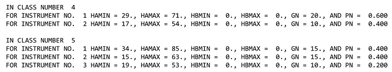
Fig. 6.2 Program output showing timbre classes 4 and 5. Figure created by author (2024).

In addition to timbre, textural density—the thickness or thinness of the instrumentation in the ensemble—is another important characteristic of the music that is managed in the Free Stochastic Music program. As in other works by Xenakis, textural density is quantified in the program in terms of the average number of sounds per unit of time. The minimum density he chose for Atrées was 0.05 sounds per second, equivalent to one sound every twenty seconds.9 He then constructed a logarithmic scale of densities, using e, the base of the natural logarithm (approximately 2.71) as the base for the scale. As the exponent for e varies from zero to six, seven levels of density are produced as shown in Figure 6.3. It should be noted that these density levels are thresholds and not the only values used in Free Stochastic Music. The actual densities produced by the program vary continuously between these thresholds.

Fig. 6.3 Levels of textural density used in Atrées. Figure created by author (2024).

The heart of the Free Stochastic Music program consists of the coupling of textural density with instrumental timbres. This is illustrated by the excerpt from the program’s output shown in Figure 6.4. The figure shows timbre classes 1 (percussion) and 2 (horn) along with the probabilities that sounds from this timbre class will be chosen for inclusion in the ensemble when the textural density of the entire ensemble falls within levels 1–7, whose precise threshold values are shown in Figure 6.3. Note that the probabilities do not vary in a predictable pattern from level to level: this is because these probabilities are assigned by the composer as part of the compositional process, likely chosen in order to generate a complex and varied instrumentation rather than a steady increase or decrease in probability for each timbre.

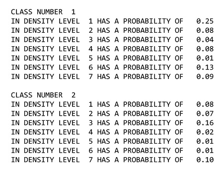
Fig. 6.4 Program output showing probabilities of sounds from timbre classes 1 and 2. Figure created by author (2024).

Once the general properties of a section have been determined—such as its length, the number of notes it will contain, and the probabilities of the timbres it will contain—the program moves on to determine the characteristics of the section’s individual notes. The image in Figure 6.5 is an annotated note list for the first section of the output from a run of the Free Stochastic Music program from 1 July 2022.10

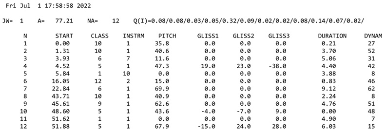
Fig. 6.5 Note list from program output (excerpt). Figure created by author (2024).

The item to the right of the value for NA is Q(I), which gives an array of values representing the probabilities of the occurrence of sounds from timbre classes 1–12. The values for timbre classes 1 and 2, both 0.08, may be compared with the values for these classes for density level 2 in Figure 6.3: 0.08 for timbre class 1 and 0.07 for timbre class 2. The match between the values for class 1 and the proximity of the values for class 2 between Figures 6.3 and 6.4 makes sense because the actual density of the section whose data are shown in Figure 6.4 is so close to the value given for level 2 in Figure 6.3. Given the slight increase in density from 0.14, the threshold value for level 2, and the density of section 1, 0.155, the probability of sounds from timbre class 1 has not noticeably begun its decrease from 0.08 at level 2 to 0.04 at level 3 while the probability of sounds from timbre class 2 has already begun its increase from 0.07 at level 2 to 0.16 at the level 3, arriving at 0.08 when the actual density is 0.155.11 A perusal of all of the values in the Q(I) array indicates that the highest values are for classes 5 and 10, at 0.32 and 0.14, respectively. These values lead us to expect a greater frequency of sounds from class 5, glissando sounds, and class 10, trumpet, than from the other classes. This is indeed the case, with occurrences of sounds from class 5 at notes 4, 10, and 12 and sounds from class 10 at notes 1, 2, and 8. Given a sample size of twelve notes, the frequency of sounds from class 5 is a little lower than expected (3/12 = 0.25 versus 0.32) while the frequency of sounds from class 10 is a little higher than expected (0.25 versus 0.14). These differences are not unexpected, however, given the small sample size of twelve notes.

A transcription of the first five notes from the note list in Figure 6.5 is shown in Figure 6.6. The first two notes belong to the trumpet (class 10, instrument 1). The pitches are the closest integer approximations of the pitches shown in the note list: note 1, pitch 36 (A3), an approximation of the given value of 35.8, and pitch 41 (D4), an approximation of the given value of 40.6. The third note is a flutter-tongue articulation on a pedal tone of the tenor trombone (class 6, instrument 7) on pitch 12 (A1). This is followed by a glissando on the violin (class 5, instrument 1) beginning on pitch 47 (G#4). (As before, the pitches are the closest integer approximations of the given values.) Three values are given for each glissando, representing three methods of calculation.12 The composer chooses one of the values. In this case, I chose the value for “GLISS2,” a rising glissando of twenty-three semitones. (Falling glissandi are shown with negative values.) The endpoint of this glissando is pitch 70 (G6), 23 semitones above the starting pitch, 47. No pitch is given for note 5, which is for maracas (class 1, instrument 10).

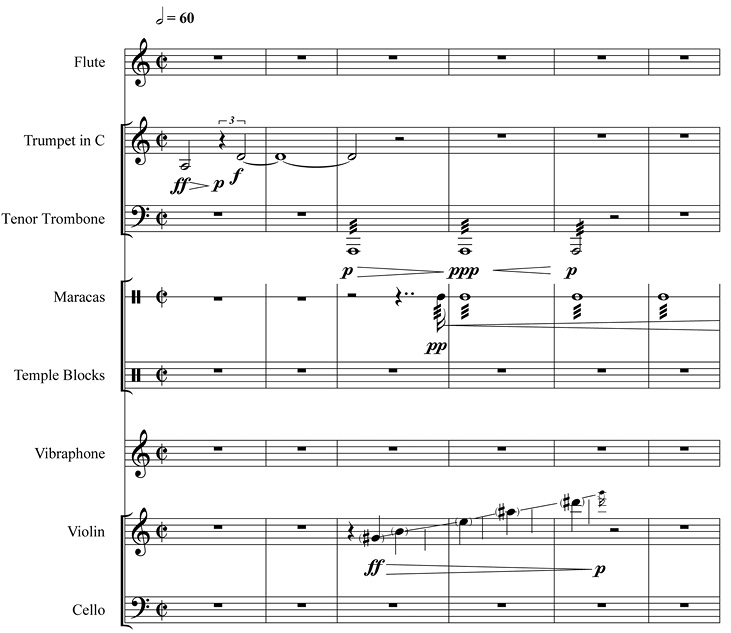
Fig. 6.6 Transcription of the first five notes from the note list in Figure 6.5. Figure created by author (2024).

The values in the column for durations give suggested note lengths in seconds, which may be increased or decreased to conform to whole numbers of beats or to their standard metrical divisions, or for other musical reasons. I have chosen to extend the duration of note 5 for maracas because there is a gap of more than ten seconds between the start of that note and the start of note 6 (not shown in Figure 6.6). The values for dynamics vary from 0 to 63, of which a representative selection is shown in Figure 6.5. The sixty-four dynamic values represent the possible combinations of four dynamic levels—ppp, p, f, and ff—taken three at a time. The table of forty-four intensity forms given in Formalized Music is a condensation of the longer list from which duplicates have been removed.13 For example, the crescendo from ppp to p, the second value on the list of Xenakis’s intensity forms, may be formed in two ways: as a succession of ppp, ppp, and p, or ppp, p, and p. Since both successions begin with ppp and end with p, they are both represented in Xenakis’s table by the same crescendo from ppp to p. The dynamic markings in the score excerpt Figure 6.6 are based on a hypothetical correlation between the values for dynamics on the program output and Xenakis’s table of intensity forms.

Toward an Analysis of Atrées

Armed with some basic knowledge of the characteristics of the output from Free Stochastic Music, we may now approach a passage from Xenakis’s Atrées analytically, focusing on the structural features that are shaped by the program’s mode of operation. Figure 6.7 shows a hypothetical note list for the first movement of Atrées which, as indicated in the score, is a transcription of the data for sections JW 1 and JW 2 of output that was produced on 6 September 1962.14

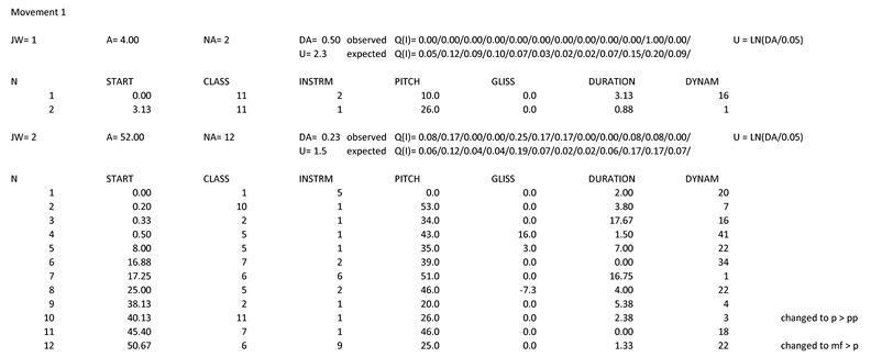
Fig. 6.7 Hypothetical note list for Atrées, movement 1. Figure created by author (2024).

There are a few differences to note between the note list in Figure 6.7 and the list in Figure 6.5. The first difference is that two arrays, Q(I), are shown for the timbre classes in Figure 6.7 rather than the single array that appears in Figure 6.5. This is because the finished composition presents an observed distribution of timbre classes that may be compared with the expected distribution that emerges from the design of the program. The variable U that appears in Figure 6.7 is equivalent to the level of density minus 1, e.g. U = 2.3 indicates that the level of density is slightly higher than the threshold for density level 3. For both sections JW 1 and JW 2, given the small sample sizes of two and twelve notes, respectively, the expected distributions of the timbre classes are reflected reasonably well in the observed distributions: where fewer notes in a timbre class are indicated in the expected distribution, fewer appear, and where more notes are indicated, more appear. This is true even for JW 1, for which the greatest number of notes is expected for timbre class 11 (trombone) and, in fact, both of the notes in this extremely brief section are for trombone. Another difference between the note lists is that pitch values are given in Figure 6.7 with only 0 after the decimal point since, unlike in Figure 6.5, the pitch values have already been rounded to the nearest integer prior to being notated in the score. In Figure 6.7 only one column of values is shown for the glissandi since only the value chosen for transcription is included in the score. Finally, the values for dynamics in Figure 6.7 match those in Xenakis’s condensed table of forty-four intensity forms.15 Two of the dynamic forms in the score—for JW 2, notes 10 and 12—are different from the prototypes in Xenakis’s table. Since the values in these dynamic forms each differ by one level from one of the prototypes, however, it is possible to associate them with the prototypes they match most closely.

What does analysis of the hypothetical note list tell us about the structure of Atrées? First, at least in the movement examined here, the association between the timbre classes and the level of density follows the program’s theoretical premises to a reasonable approximation. Second, looking at Atrées and the other works in the computer-generated stochastic corpus more broadly, Xenakis’s judicious choice of which sections of music to transcribe and assemble into finished compositions resulted in varied, aesthetically engaging works. Within these works, the variations in textural density, along with their associated blends of timbre, made for a satisfying degree of contrast and variety on the musical surface. In this respect, the thesis that drove Xenakis’s development of this approach to composition was borne out in the final results.

Further exploration along the lines of what has been demonstrated briefly here, using Atrées as a test case, may confirm that the compositional implementation of timbres as a function of density remains fairly faithful to the expected distributions that are inscribed into the Free Stochastic Music program throughout the composition. Once an examination of hypothetical note lists for the remaining movements of Atrées has been accomplished, its general musical characteristics—melodic, harmonic, and rhythmic—may be analyzed independently of the theoretical premises of the program. General analysis of this kind will allow the structural features of Atrées and other works from the Free Stochastic Music corpus to be compared to works by Xenakis and others that proceed from different theoretical premises.

MYHILL, John (1978), “Some Simplifications and Improvements in the Stochastic Music Program,” International Computer Music Conference Proceedings, vol. 1978, p. 272–317, http://hdl.handle.net/2027/spo.bbp2372.1978.023

ROGERS, Bruce (1972), “A User’s Manual for the Stochastic Music Program,” Senior honors thesis, Indiana University.

TURNER, Charles (2014), Xenakis in America, Tappan, New York, One Block Avenue.

XENAKIS, Iannis (1963), Musiques formelles, Paris, Richard-Masse.

XENAKIS, Iannis (1965a), “Freie stochastische Musik durch den Elektronenrechner,” Gravesaner Blätter, vol. 26, p. 54–78.

XENAKIS, Iannis (1965b), “Free Stochastic Music from the Computer,” Gravesaner Blätter, vol. 26, p. 79–92.

XENAKIS, Iannis (1968), Atrées pour onze instruments (score EFM 836), Paris, Salabert.

XENAKIS, Iannis (1971), Formalized Music: Thought and Mathematics in Music, Bloomington, Indiana, Indiana University Press.

XENAKIS, Iannis (1992), Formalized Music: Thought and Mathematics in Music (rev. ed.), additional material compiled and edited by Sharon Kanach, Stuyvesant, New York, Pendragon.

XENAKIS, Iannis (2010), Achorripsis, Akrata, Atrées, Herma, Morsima-Amorsima, Nomos Alpha, Polla ta Dhina, ST/4, ST10-080262. Instrumental Ensemble of Contemporary Music, Paris, Konstantin Simonovich (dir). EMI Classics CD 6 87674 2, “Xenakis: Chamber Music”.

References

CHIVERS, Ian and SLEIGHTHOLME, Jane (1981), Introduction to Programming with Fortran (2nd ed.), London, Springer.
HEALY, Jeremiah and DE BRUZZI, Dalward (1975), Basic Fortran IV Programming (rev. ed.), Reading, Massachusetts, Addison-Wesley.
IBM DATA PROCESSING DIVISION (1960), “7090 Technical Processing System” [fact sheet].
MCLEAN, Alex and DEAN, Roger T. (eds.) (2018), The Oxford Handbook of Algorithmic Music, New York, Oxford University Press.