
13. Code against code: Creative coding as research methodology
Cameron Edmond and Tomasz Bednarz
© 2024 Cameron Edmond and Tomasz Bednarz, CC BY-NC 4.0 https://doi.org/10.11647/OBP.0423.13
Abstract
Machine writing—where computing methods are used to create texts—has risen in popularity recently, diversifying and expanding. Machine writing itself could be seen as a subset of the creative coding discipline. Emblematic of the contemporary turn in machine writing is Darby Larson’s Irritant. Impenetrable by traditional reading standards, the text is governed by code. The reader of Irritant faces similar challenges to the Digital Humanities scholar attempting to analyse large textual corpora. As such, Irritant becomes a useful case study for experimenting with reading methodologies.
We approach Irritant from a computational criticism perspective, informed by the same creative coding methods that spawned it. Our objective is to reverse engineer Irritant, scraping its repetitions and variables using Python within a live coding environment. We position creative coding as a research methodology itself, especially suited for analysing machine-written texts.
This chapter details our process of back-and-forth iteration between the researcher and the text. The ‘hacking’ of the text becomes critical practice itself: an engagement with the coded artefact that meets it on even ground. What our analysis finds, however, is more questions. Our exploration of Irritant fails to unravel the novel’s code in the way we planned, but instead reveals more thematic depth. Far from the post-mortem of a failed experiment, this chapter presents creative coding as a research methodology and interrogates its benefits and challenges via the Irritant case study.
Keywords
Machine-writing; distant reading; graph theory; algorithmic literature; creative coding.
Introduction
In something of red lived an irritant. Safe from the blue from the irr. And this truck went in it. Safe. Something of red in it back to the blue to the red. This truck and something extra (Larson, 2013, p. 1).
So begins Darby Larson’s monolithic text Irritant (2013). And so it continues, winding through surreal, asemantic statements that challenge reader comprehension. Irritant represents the creative coding practice of machine writing, where computing methods are used to create texts (Edmond, 2016, p. 4–5). As a textual practice, machine writing has experienced renewed interest within both popular (Heflin, 2020) and academic discourse (Orekhob, 2020). A lingering question of these interrogations is what methodologies are best suited for analysing machine-written texts, especially those generated from large textual corpora (Fullwood, 2014) or that are interactive (Walton, 2019). In this context, Larson’s Irritant is an interesting beast. Irritant’s construction is far more simplistic, using simple generative and cut-up methods akin to William S. Burroughs and the Dadaist movement (Robinson, 2011, p. 1–20). However, the abrasive prose of Irritant defies traditional reading standards. Rather than a traditional, temporal narrative, Irritant treats the text of the novel more like a texture. A single, monolithic paragraph is repeated, with each repetition featuring slightly altered sentences with objects, characters and actions changed. These actions are incremental, causing a slow rise and fall of these entities and actions throughout.
Despite its form, one could take a linear approach to reading Irritant. However, the veracity of such a reading is questionable. While the theme of relentless, linguistic oppression will be apparent, making sense of anything else requires a more systemic approach, one that can find the mutations within the sea of sameness. This observation leads us to inquire as to whether the computational criticism of the Digital Humanities (DH) can help us make sense of machine-written texts.
Analysis of machine-written texts has existed within fringe groups of literary scholarship for some time. Attempts to unravel texts produced via automation date back to at least the early 1980s, when computing and tech journalism began to show interest in computational texts (Edmond 2019, p. 37). However, recent years have seen an uptick in the relevance of machine-written texts. Writing in 2023, the most recent of these developments is the proliferation of Large Language Models (LLMs) such as OpenAI’s ChatGPT, which some users have used to generate novels (Coetzee, 2023). At present, it seems that this form of Artificial Intelligence (AI) tool—one that produces text that bears extreme similarity to that of the human—is only likely to become more pervasive throughout our society.
Any grievances or jubilations about the world of Generative Pre-trained Transformer (GPT) texts aside, as the textual possibilities of AI continue to extend into new directions, it is important for us to understand how we may ‘read’ a text that is truly machinic. The productions of these LLMs are vastly different from Larson’s Irritant. A foundational understanding of how one might speak to ‘code through code’ is important for the DH researcher of the future, and we believe doing so on the level of the machine—rather than when it is trying its hardest to appear human—may be the best way to get there.
While many DH techniques and tools are developed for the programmatic interrogation of texts at large, we are instead proposing a close reading. Our approach is not without precedent, as evident in the Z-Axis Tool that transposes literary works into 3D maps (Christie and Tanigawa, 2016). However, the Z-Axis Tool is only useful to a reader who knows what they are looking for—that is, the relevance of particular locations. Arguably, the reader of Irritant is starting from a somewhat less secure position, knowing only that the text they are stepping into is literally (and literarily) inhuman. Consequently, our attention turns to Jan-Hendrik Bakels et al.’s (2020) tool for computational visualisation/annotation of films, which they refer to as a “systemic approach to human experience” (par. 12). One of the solutions the team demonstrates involves the creation of a timeline of the media in question, complete with the audio visualised as a waveform. The resulting view is akin to what a post-production professional would view when working on a film, mimicking the process of creation and allowing the user to peer ‘behind the curtain’ of the artefact.
Following Bakels et al.’s (2020) lead, we approach Irritant with a similar deconstructive approach in mind. As Larson’s text was constructed through methods of creative coding, we will attempt to use similar techniques to analyse the text. In doing so, we offer a case study into the effectiveness of creative coding as a research methodology. Our initial analysis set out to unravel the code of Irritant itself. However, as we plunged deeper into the text, we were left with more questions. Our analysis revealed to us new thematic avenues and possibilities, thereby shedding light on both Irritant and how researchers may wield creative coding to conduct research.
Our work is also aligned with several other DH practitioners currently active in this field. John Mulligan’s ‘middle-distant’ form of reading has recently examined the tensions that exist between numerical analysis and literary theory and attempts to reconcile the two.
Furthermore, the twisting and deforming of text to divine further meaning is a practice we are certainly not pioneering. Lisa Samuels and Jerome McGann (1999) discussed the reading of a text “against the work’s original grain” (Samuels & McGann, 1999, p. 28). While discussing poetry, the pair suggest a new mode of critique: do not ask what the poem means, but instead investigate how you can release and expose this meaning.
Attempting to further pinpoint all the methods influencing this practice would be a chapter in and of itself. Instead, we point towards James E. Dobson’s (2019) overview of the landscape of DH reading methods. Here, Dobson discusses the concept of “surface reading”, and its relationship to approaching a text without a lens of “superstition” that accompanies close reading. Indeed, many of the practices we utilise emerge within such surface-reading approaches, down to the use of Python and Jupyter Notebooks. However, we approach our study with a far different intention. While a surface-reading approach may suggest meaning sits within the text, awaiting discovery, we instead recognise our programmatic reading as a sort of close reading itself, but simply one through a different method. We have, to put it crudely, replaced our pens and margin notes with loops and arrays. Our approach is deliberately inhuman, for what we are reading is as well.
Finally, we must address that while our methodology encourages the writing of code by the critic, our enquiries and practices may also apply to other existing tools for those apprehensive about starting programming themselves. Tools such as Voyant Tools and Omeka allow the visualisation of formalist textual elements, as well as marking up and annotating them. For those unsure where to begin, we suggest these tools as a starting point along their journey.
Creative coding
Traditionally trained artists are increasingly interested in coding, as is evident in the proliferation of tools designed to facilitate the field of creative coding directly, such as Stamper (Burgess et al., 2020), and texts written to introduce arts practitioners to coding (Montfort, 2016). However, there is an erroneous narrative that computational art came about post-1980s. Artut (2017) states that it was only “a limited group of engineers and scientists who became experts in computer programming” (p. 2). While Artut’s (2017) statement that computing was less accessible during the 1980s is true, it oversimplifies the use of computation in artistic practice, which dates back to at least Christopher Strachey’s Love Letter Generator (Wardrip-Fruin, 2005), and glosses over the demoscene (Hansen et al., 2014), arguably a precursor to contemporary creative coding.
Creative coding has been referred to as decidedly iterative and reflective, likened to the painter who makes some expressions on the canvas and then decides what to do next (Bergstrom and Lotto, 2015, p. 26). Essentially, planning is reduced if not eliminated. Bergstrom and Lotto (2015) extend this metaphor by describing “live coding” in which individuals write code in front of an audience (pp. 26–27). The pair also associate creative coding with hacking. Nikitina (2012) describes hackers as the tricksters of the digital age, performing inventive, barrier-crossing tasks that leverage systems in the search for creativity (pp. 133–135). Much like the trickster of mythology, the hacker manipulates the systems around them to alter their environment. Their subversion becomes their artistry. In keeping with these sentiments, our definition of creative coding encompasses the need for the act to be an iterative ‘hacking’ away at the subject.
Without planning too far ahead, we do need to consider what we wish to uncover from Irritant. Given its algorithmic form, the patterns themselves are a good starting point. This leads us back to the techniques that bore Irritant initially: textual manipulation. Our starting point, then, is to try and unravel the repetitions and variables of Irritant. As we wish to do so iteratively and reflectively, we will use a Jupyter Notebook. A Jupyter Notebook is a live programming environment, that allows users to write blocks of code and execute them as they go, creating a space for exploratory and iterative programming (Project Jupyter). Notebooks can be shared, so ours is available from http://hci.epicentreunsw.info/creativecode.html. While we cannot upload our source material, by making our code available, we hope to encourage readers to experiment with the code in their analysis of other texts.
A note on the syntax and style of code used in this chapter. While completed code is often re-factored to appear more beautiful, function better and achieve more reliable results, our purpose here was to show the live ‘hacking’ experience of attempting an enquiry, learning from the result (or error message) and trying again. As such, while we stand by the methodology presented here, we make no such claims about the styling and formatting of the code. Please view the actual code presented here as scribbles in the margins, rather than completed analysis.
Prep time
Machine writing texts such as Irritant are, in many ways, ‘hacks’ of language and literary tradition. As illustrated in the yearly submissions to NaNoGenMo (Kazemi, 2013), to practice machine writing is to play with language. Although some scholars have studied Irritant (Sierra-Paredes, 2017; Murphet, 2016) the question remains: how do we unravel this enigma? What is the key to opening the monolith and discovering the meaning within? We view it as a puzzle: a dense tome that challenges the reader. We must follow the clues and construct the jigsaw piece by piece, forming the picture as we go.
Larson is not the first to craft a puzzle for their reader in the form of unconventional discourse. Life: A User’s Manual (1987) by Georges Perec refers to itself as a jigsaw puzzle in its opening pages. Similarly, as the brain in Plus (2014) by Joseph McElroy relearns consciousness, the reader is invited to piece together the story. However, McElroy and Perec both give the reader more clues as they go. By sheer dint of perseverance, the reader will find answers by the time they reach the final page. For the reader of Irritant, there is no such certainty. Irritant ends much as it began: the monolithic paragraph iterates a few more times and ends—almost mockingly—with the statement “this is a showboat” (Larson, 2013, p. 623).
However, Larson has left clues for those trying to solve Irritant. In an interview, Larson presented the code used to generate the short story “Pigs”, in which a series of sentences slowly evolve, their original words being replaced with a litany of other nouns, creating a textual unravelling (Larson, “Pigs”). Larson then suggests that “similar” constraints were used to create Irritant, stating the original idea as “a 70-word initial set that slowly changes to a completely different 70-word final set with a one-word change occurring every 4000 words. So, 4000 x 70 is 280,000 words total” (Butler & Larson, 2013). Larson cryptically continues:
Irritant ended up being quite less than 280k […] I wrote the first 4000 words on my own, just stream of consciousness while referring to the word set. Then I randomized that and concatenated it to the original (so now 8000 words) and did one-word substitution on the new 4000, and so on and so on until all 70 words had been substituted (Butler & Larson, 2013).
From Larson’s statement, we can begin to unravel Irritant armed with the following clues:
- The first 4000 words are completely humanly written.
- The second 4000 are randomised.
- There are 70 words that become substituted.
These points are useful, but also establish the difficulty of our task. The core of Irritant being written by a human rather than a machine throws it into a nether realm of study. A human-penned puzzle has its pieces placed deliberately, ready to be solved. Further, a completely machinic text would require only one cracking of the pattern to uncover its workings. Irritant sits between the two worlds, guarded by both humanity and machinery.
The first step, then, is to check the veracity of Larson’s claim. According to the copy of the text we have, Irritant’s word count is 272,267. If an iteration occurs every 4000 words, and accounting for the novel’s first 4000 words being ‘outside’ the equation and the next 4000 being iteration zero, we are left with 264,267 words (272,267 – 8,000). Dividing this by 4000, we are left with 66.1, three (and change) words shy of Larson’s claimed 70 iterations. We then must ask: did Larson begin counting his iterations earlier? Did he use some sort of post-processing to remove sections that weren’t interesting? And how do we account for the stray 267 words, which based on initial sums do not fit nicely into our calculations? Larson has likely both made a few tweaks in the editing room and, perhaps, forgotten the exact number of iterations contained in the book. Taking these two points as our preliminary hypothesis and armed with a digestible version of the text ready to ‘hack’, we begin our spelunk into the literary depths of Irritant.
Hacking Irritant
The text of this chapter is written to present our methodology in a way that it can be reproduced. As such, we assume very little of our reader’s knowledge of the Python language. However, if for no other reason than chapter length, we will not be delving into how to install Python or Jupyter Notebook. Thus, our process begins at the step of having digested Irritant’s text into a .txt file and opened up a Python 3 Jupyter Notebook to begin our excavation. We first import all necessary libraries and then turn our .txt file into a single string.
|
import pandas as pd import nltk from nltk.stem.wordnet import WordNetLemmatizer as WL from statistics import median import matplotlib.pyplot as plt with open ("irritantraw.txt", "r") as irr: irritant = irr.read() |
We now have our subject in a raw, textual form for processing. There are many starting points here. Given Larson’s discussion of word permeation, we will first uncover exactly what words appear throughout the text by creating a list of every unique word within it. We create a version of Irritant that removes punctuation and capitalisation to make it easier to split into words and avoid false positives. We then transform this string into a list of all words in Irritant.
|
punctuation = [".",",","?","!"] irritant_np = irritant for p in punctuation: irritant_np = irritant_np.replace(p,"") irritant_np = irritant_np.lower() irritantlist = irritant_np.split(" ") |
This list will certainly include duplicates, so from here we generate our new list of ‘prime’ words, which includes each word only once.
|
irritantwords = [] for word in irritantlist: if word not in irritantwords: irritantwords.append(word) print(word) |
This gives us our list of every word within Irritant—a total of 478 unique words. If we still believe Larson’s original claims, this leaves us with (478-70*2=) 338 ‘generic’ words that do not evolve over the course of the system. We can assume these words are most likely articles and conjunctions, although we cannot prove this yet. Another step is to see just how many times each word appears. Because we kept both lists, we can compare them and retrieve the count of each unique word.
|
for word in irritantwords: count = irritant_np.count(word) print ("There are " + str(count) + " instances of '" + word + "' in total.") |
Although this method allows us to produce a plain, textual list of each word and its frequency, a list of 478 words is only marginally more readable than Irritant itself, and, on its own, it will not reveal much. It would be better to visualise this data. First, we will need to place unique words and their counts into a tabular dataset/dataframe. As we will be doing this a few times, we will write a function to create our graph. After a run, it became clear that visualising all 478 words was unwieldy, and it might be better to begin with the top 50 and bottom 50 words, amalgamated in Figure 13.1.
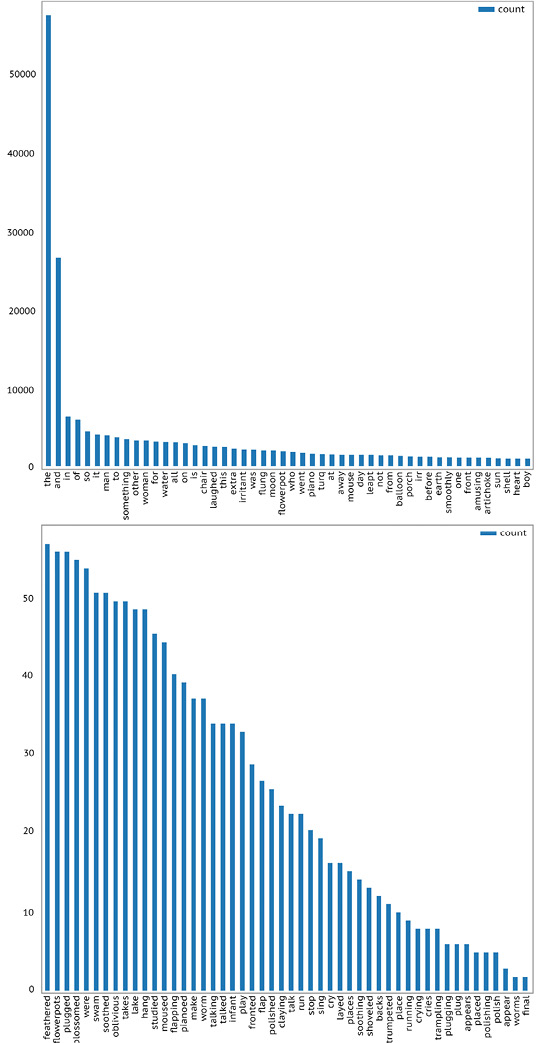
Fig. 13.1 The top and bottom 50 words in Irritant, sorted by frequency.
|
def visualise(uniquewords,fullcorpus): wordcount = [] for word in uniquewords: count = fullcorpus.count(word) wordcount.append(count) df = pd.DataFrame({'word': uniquewords,'count':wordcount}) dfsorted = df.sort_values(by='count', ascending = False).head(50) dfsorted.plot.barh(x='word',y='count', figsize=(30,30), fontsize=20) dfsorted = df.sort_values(by='count', ascending = False).tail(50) dfsorted.plot.barh(x='word',y='count', figsize=(30,30), fontsize=20)
visualise(irritantwords,irritantlist) |
Looking at our top 50 words, it becomes abundantly clear that the inclusion of our generic terms—especially “the” and “and”—is obfuscating any insights. Our next step, then, is to shrink our list down so we can examine only the evolving words. There are a handful of ways we could do this. We could guess which words are generic, but we will likely miss some, making this a time consuming and error-prone method. We could comb through the text itself and find words, but this would defeat the purpose of our hack-based reading methodology. Most other solutions involve bringing in some sort of NLP library, in this case, NLTK, that offers some intelligence as to how words hang together.
First, we will try using NLTK to analyse the text and find what words are similar to one another. This should give us a good idea as to how the patterns of the text hang together. We begin by tokenising our text to make it readable to NLTK.
|
text = nltk.word_tokenize(irritant) irritanttagged = nltk.pos_tag(text) context = nltk.Text(word.lower() for word in text) |
Through this method, we should receive a list of every word used in similar settings to the eponymous “irritant”, one of the words we propose is evolving throughout the text. We run the code “context.similar(‘irritant’)”, which returns “woman porch water morning moon turq chair other evening man sun balloon corner door kitchen artichoke weather flowerpot infant blue”. This isn’t particularly insightful. While it does indicate we are on the right track (nouns appear to be replaced by nouns), it is hardly a conclusive list. Moreover, running the query on “the” (“context.similar(‘the’)”), yields a few of the same words, such as “moon”.
While these results are discouraging, they do create some inroads into Larson’s linguistic puzzle box. If “the” and “irritant” share similarities, this implies that Larson’s pattern does not follow a traditional syntactical pattern. So, we will now see if we can retrieve all nouns and verbs from the text to map what structure does exist. NLTK can help us do this, as it tokenises and tags words based on their lexical role. For instance, conjunctions are tagged with “CC”, common nouns with “NN”, proper nouns with “NNP”, etcetera. Following the creative coding mantra of “leap before you look” (Greenberg et al., 2013, p. xxiii), we will begin by creating a new list of all nouns, pronouns, adverbs and verbs. To start, we first want to get a lead on what tags are present in the text, so we don’t waste time having our code look for tags that don’t appear.
|
alltags = [] for word, tag in irritanttagged: if tag not in alltags: alltags.append(tag) print (tag) |
An interesting observation is that when our script returns the list, it includes “FW”, which NLTK assigns to non-English words.79 By probing what this word is:
|
for word, tag in irritanttagged: if tag == "FW": print (word) |
It is revealed that the word is “masked”, rather than the far more likely invented words of Irritant, such as “turq” (a contraction of turquoise, perhaps?) and “elbowthumbs” (an impossible body part?). This exercise reminds us of the limitations of our method. The delegation of “masked” as “foreign” aside, we can use this information to generate a much shorter list of words and get closer to understanding how Irritant’s patterns manifest. Firstly, we define a function for simplifying words to avoid repetition. At the moment, all this function will do is change a word to lower case and add it to our working ‘evolving words’ list.
|
def simplify(word, targetlist): word = word.lower() if word not in targetlist: targetlist.append(word) |
We then identify all tags we wish to keep and simplify the associated words.
|
goodtags = ['NN,','JJ','VBD','PRP','NNP','RB','NNS','VBN','VB','PDT','VBG', 'PRP$','VBP','VBZ','RBR','JJR','UH','JJS','FW'] evolvingwords = [] for word,tag in irritanttagged: for gt in goodtags: if tag == gt: simplify(word,evolvingwords) print (evolvingwords) print (len(evolvingwords)) |
The resulting list is not perfect, coming in at 332 words and featuring several duplicates in the form of plurals and different tenses. We test its use by first running it through our word count function from earlier (“visualise (evolvingwords,irritantlist)”). Our resulting graphs were better, but a few words have slipped through the categorical cracks, such as “is” and “as”. We can quickly remove them and run our code again: the results are depicted in Figure 13.2. Interestingly enough, this level of manual editing moves us closer to Larson’s practice, as he made a few changes to his output. However, we are still maintaining a computational slant by not directly deleting data points and instead using scripting to do so.
|
badwords = ['is','as','so','it'] for bw in badwords: evolvingwords.remove(bw) visualise(evolvingwords,irritantlist) |
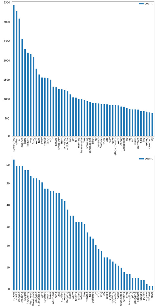
Fig. 13.2 The top 50 and bottom 50 of our “evolving words” in Irritant, sorted by frequency.
Our resulting visualisations show a lot more promise. The most common word in the text appears to be “something”, indicating that it either never evolves, or is the final piece to do so. “Irritant”, “irr” and “irrd” all make the top 50, which is unsurprising. The absence of “red” is interesting. The novel’s opening would make it seem that “red” will feature prominently. Instead, “blue” steals the show.
It is here we start to question what constitutes a unique ‘word’ in Larson’s pattern. Are “cough” and “coughed” unique permeations, or the same permeation but with the tense skewed either by code or by Larson’s hand? If the former, then the permeations are greater than Larson stated. If the latter, then having a list to access the permeations directly would go a long way towards unravelling Irritant. We could achieve this by reducing each instance to its base form. NLTK can achieve this via the “lemmatize()” function. Adding this to our simplify function has unintended consequences, as it converts “went” to “go”, “ground” to “grind” and a few other transformations that make our list too divorced from the original text to be useful. Perhaps we need to flip the script and search for the words around the permeations. We fall again to our creative coding mantra of experimentation and attempt to retrieve some sort of ‘boilerplate’ of Irritant. We first create a new list of every sentence.
|
badpunctuation = ["?","!"] irritantcleaned = irritant for bd in badpunctuation: irritantcleaned = irritant.replace(bd,".") irritantsentencelist = irritantcleaned.split(". ") for sentence in irritantsentencelist: print (sentence) print (len(irritantsentencelist)) |
We then filter this down to just the unique sentences.
|
irrusentences = [] for sentence in irritantsentencelist: if sentence not in irrusentences: irrusentences.append(sentence) print (sentence) print (len(irrusentences)) |
While the novel contains 20,724 sentences, only 1612 of these are unique. This leaves us with 19,112 repetitions throughout the novel. This is interesting, as a cursory look over Irritant gives the appearance that sentences change constantly, if only slightly. We will return to this number soon, but first we want to finish what we started and try to find the boilerplates of the text, replacing each evolving word with “<BLANK>”.
|
boilerplates = [] irritantcleanlist = irritantcleaned.split(" ") irritantnewlist = [] evolvingwords_punctuated = [] missedwords = ["flowerpot", "chair", "porch", "truck", "carpenter", "door", "shell", "piano", "kitchen", "showboat", "hearth", "balloon", "woman", "moon", "man"] for mw in missedwords: evolvingwords.append(mw)
for word in evolvingwords: evolvingwords_punctuated.append(word + ".") for word in irritantcleanlist: if word in evolvingwords or word in evolvingwords_punctuated: irritantnewlist.append("<BLANK>") else: irritantnewlist.append(word) irritant_boilerplated = " ".join(irritantnewlist) boilerplates = irritant_boilerplated.split(". ") boilerplates_unique = [] for sentence in boilerplates: if sentence not in boilerplates_unique: print (sentence) boilerplates_unique.append(sentence)
print (len(boilerplates_unique)) |
As we peruse our results, it becomes clear that certain obviously evolving words such as “flowerpot” have evaded NLTK’s categorising. The results are noisy, and don’t seem to show any patterns. Our hypothesis of some ‘generic’ words and some ‘non-generic’ words may have been inaccurate. Perhaps all words are permeating. If so, what method is keeping these sentences ‘in check’? Perhaps reducing each sentence to its semantic NLTK tags will help shed our text of any noise.
|
justtags = [] for word, tag in irritanttagged: justtags.append(tag) irritanttags = " ".join(justtags) irritanttagsents = irritanttags.split(". ") for sent in irritanttagsents: print (sent + " ---------> " + str(len(sent.split(" ")))) |
Still no discernible patterns seem to emerge. Word type and sentence length are arbitrary, with no overarching patterns. While this might be discouraging, it is par for the course: our philosophy of hacking away at this novel has already dramatically changed our understanding of how it works. Larson’s claims seem to be completely false, or else made obsolete by his human-level tampering. Instead, the abstracted, hacked artefact of Irritant is forming into something far different. But we aren’t done yet.
While we are unable to find patterns on this macro level, due to the difference in size between our complete sentence list and our unique sentence list, we know there is repetition. So, how often does a new sentence manifest? We can better understand this by visualising it, charting each period of repetitions and how many sentences repeat between them.
|
repeatcount = 0 repeats = [] periods = [] periodcount = 0 newsentences = [] irritantsentencelist = irritantcleaned.split(". ") for sentence in irritantsentencelist: if sentence not in newsentences: if repeatcount != 0: periodcount += 1 periods.append(periodcount) repeats.append(repeatcount) repeatcount = 0 newsentences.append(sentence) else: repeatcount += 1
df = pd.DataFrame({'period': periods, 'length':repeats}) ax = df.plot.barh(x='period',y='length', figsize=(20,500), fontsize=20) |
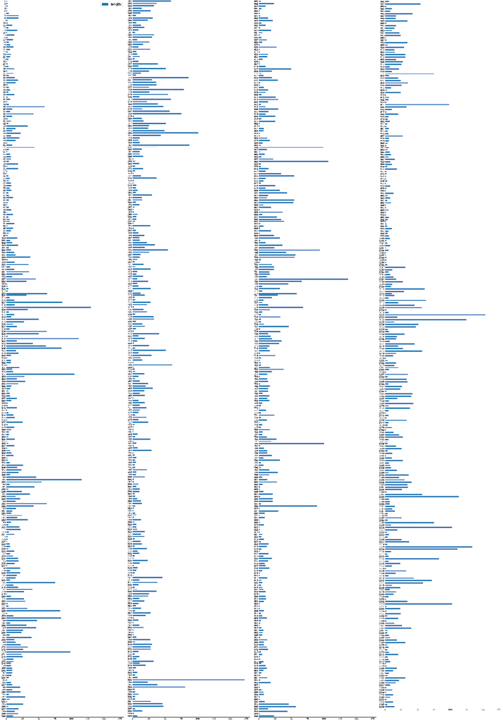
Fig. 13.3 All intervals between new sentences in Irritant and their lengths. Each column represents 300 intervals.
The result is depicted in Figure 13.3, which we have cropped and edited for readability. The resulting graph shows us that the intervals fluctuate in length, but overall become longer as the text continues. Many short intervals are slowly littered with longer ones, peaking at the 585th mark and slowly shrinking again, with the final few intervals shorter than the first bout. What does this tell us about Irritant? Sierra-Paredes (2017) refers to the “slow rhythm” (p. 31) of Irritant created by its repetitions. However, this rhythm is hard to discern. Via our visualisation, it becomes manifest.
The themes represented by the irritant itself are becoming clear. There are over sixteen intervals in Irritant where the gap between new sentences is over 100, with the largest gulf between repetition and permeation being 157. The maelstrom of repetition and monotony, disturbed by the spectre of allegory, that the reader must endure between each glimmer of newness is quantified. Due to such a high degree of repetition, we are left to wonder if most readers would even be aware of when repetitions were occurring. In effect, the clarity of our visualisation makes Irritant’s obscurity more evident.
There is one last process we wish to perform. It is likely that all words permutate, and that Larson’s clues were red herrings. However, we are still interested in when some of the more prominent words appear. Perusing our earlier lists and counts, we notice that the “infant”—a symbol for the future and a linguistic warping of “irritant”—erupts into the text towards its end. Perhaps more meaning lies in mapping some of the other terms, plucking them from the maelstrom of conjunctions and articles to better understand the presence of flowerpots, women, blue and even the irritant itself.
We initially experimented with visualising the occurrence of each evolving word per sentence, but with over 20,000 sentences (retrieved via “print (len(irritantsentencelist))”), it would be difficult to meaningfully visualise within the Jupyter notebook environment. Additionally, each word is only going to appear in a sentence once or twice, meaning any visualisation is going to be one of many ups and downs, without a clear view of how words rise and fall on a meaningful scale. We return to Laron’s clues and divide Irritant into “chunks” of 4000 words, yielding 69 chunks in total.
|
span = 4000 irritantchunks = [] for i in range(0, len(irritant_np.split(" ")), span): irritantchunks.append(irritant_np.split(" ")[i:i + span]) print(len(irritantchunks)) |
This code creates 36 graphs, which together act as a sort of summary of the novel. Unsurprisingly, some of these “scenes” are more interesting than others. In our first plot (Figure 4), “extras” has many mentions early on, but then drops off dramatically before we hit 10 chunks. “Safe” meets a similar fate, although it never had much power to begin with. “Red” has a few in the early chunks and then disappears before we get to chunk 20.
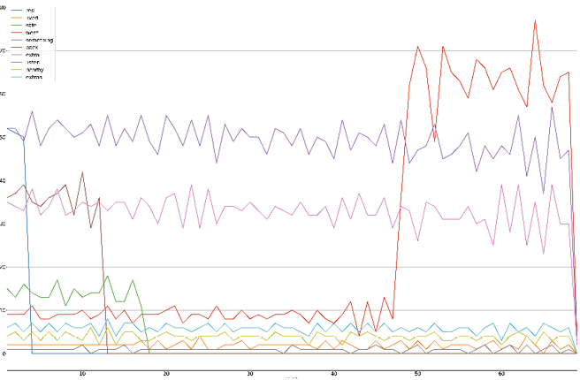
Fig. 13.4 Our first-word progression plot, depicting the words “red”, “lived”, “safe”, “went”, “something”, “back”, “extra”, “listen”, “nearby” and “extras”.
Of course, the novel’s namesake is worth interrogating. As shown in Figure 13.5, the irritant entity makes it through almost the entire novel. Far from the most popular entity, the irritant lurks within the permutations, popping up here and there, occasionally announcing itself before slinking back into the darkness. Much like the reader’s search for resolution, the “irritant” itself is just out of reach, skulking between linguistic twists and turns. In our graph, however, we do see some resolution: the irritant disappears towards the end of the novel completely, dropping to zero appearances before all is said and done.
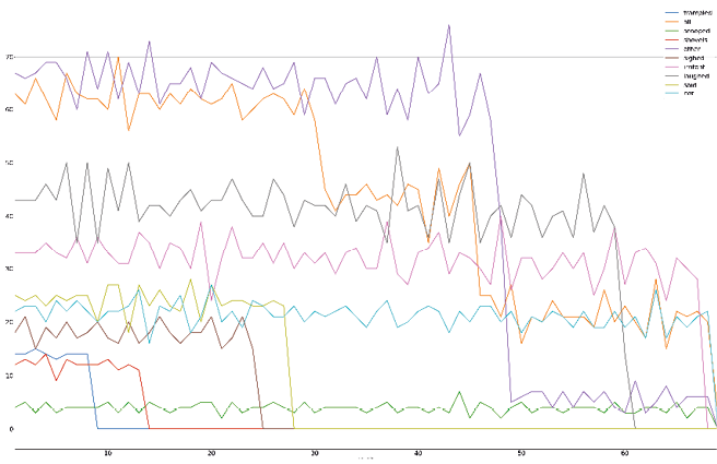
Fig. 13.5 A plot that shows the frequency of “irritant” throughout the novel.
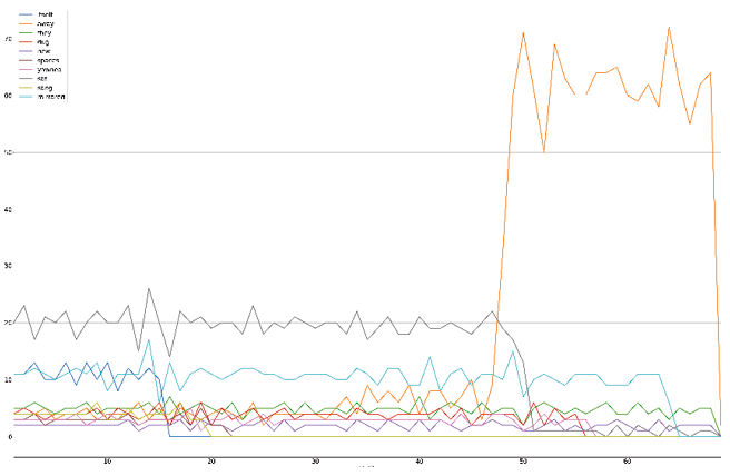
Fig. 13.6 A plot showing the frequency of “away”, illustrating how it dwarfs the terms it was featured with.
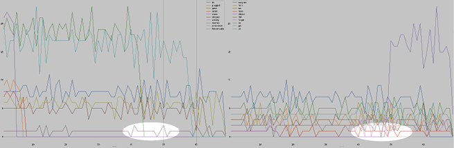
Fig. 13.7 Two plots showing the similar patterns of “have” and “seemed”, which have been spotlighted for clarity.
Some patterns emerge that may simply be red herrings. “Away” dwarfs the words it is visualised with (Figure 13.6) but may not seem so mighty if grouped with others. As Figure 13.7 shows, “seemed” and “have” feature similar patterns between chunks 40 and 50, but is this at all noteworthy? While some instances show large intervals between our word lines, others bunch together, creating interesting patterns, as seen in Figure 13.8.
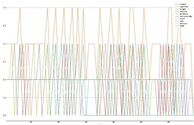
Fig. 13.8 A plot showing the interesting pattern that emerges when the frequencies of “fronted”, “expected”, “sought”, “crashed”, “trembled”, “exasperatedly”, “entire”, “well”, “returned” and “feels” are featured together.
These visualisations illustrate the importance of filtering our data. As a final visualisation, we take 10 words that we believe—together—will tell us more about Irritant. The words chosen are “irritant”, “infant”, “finally”, “weeping”, “digest”, “clay”, “whispered”, “slammed”, “cried” and “showboat”, as displayed in Figure 13.9. Comparing these words tells the story of Irritant: we see the irritant persist throughout, suffering a dip about a fifth of the way into the text, but then rising again multiple times. Ultimately, however, the irritant falls, eclipsed by the infant. In the background, the nature of the world is changing: the world of clay is replaced by one of whispering and slamming, emotions running high before the outburst of crying that usher in the infant’s arrival. A dangerous and primordial (clay) world is replaced with one of new beginnings and emotional relief. Meanwhile, a Greek choir of weeping and showboats bubbles beneath the surface, almost unnoticed throughout. Of course, this is the showboats’ plan, appearing as the final word of the text, and thereby one of its most memorable.
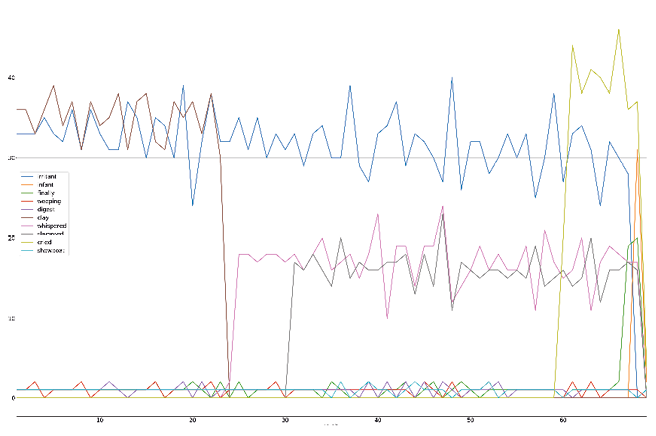
Fig. 13.9 Our final visualisation of Irritant, comparing the frequencies of “irritant”, “infant”, “finally”, “weeping”, “digest”, “clay”, “whispered”, “slammed”, “cried” and “showboat”.
Conclusions
Our final plot, while interesting, is simply one interpretation. Were we to select a different set of 10 words, we would be presented with a far different story. Our visualisation of the irritant yielding to the infant, along with our other visualisations, word counts and missteps along the way, provide us insight into how creative coding may function as a method of close computational criticism. We conclude our experiment yielded a form of analysis that was both interpretive and performative.
As an interpretation, our methodology provides an additional layer. We become divorced from the text proper, with our visualisations becoming the actual texts that we ‘read’ and interpret. However, this act of interpretation is preceded by many more interpretations. Every time we choose a method of representation or retrieve data, we are making a judgement as to what elements are relevant. If our analysis had begun with a shorter or longer list of ‘evolving words’, we may have ended up with far different conclusions. This extra layer is useful but has its flaws. As the reader explores the text through abstraction and selection, elements may be lost or forgotten. Of course, we can always return to the initial text, but it certainly suggests one can become ‘lost’ within their quantified text. We should consider the ramifications of representation when conducting these changes. Could a reader inadvertently erase the stories of marginalised groups within a text through these methods, with their resulting plots distorting the messages of the original text? The problem is not indomitable, but we must be wary not to let abstraction obfuscate the original text.
As a performance, the breakdown of the text and its abstraction is a sort of live sculpting. The original text, as data, is honed and reformed multiple times, revealing its different textures and contours with each iteration. We align ourselves here with the philosophy behind LitVis, a data visualisation tool created to allow data communicators to iterate on their visualisations, reflecting as they go (Wood et al., 2018). This chapter is a testament to that, acting as a sort of memoir of analysis, containing observations and reflections alongside findings. Returning to our hacker concept, the creative coding critic becomes the trickster of mythology, the text itself their sphynx, labyrinth, or gorgon. In truth, a creative coding methodology needn’t be performative, but simply presenting the resulting visualisations does little to advance knowledge of the text. Indeed, we hope this chapter has contributed knowledge on Irritant, as well as the use of computational mechanisms to deconstruct a text itself.
Creative coding is itself, a creative practice. As our analysis has shown, this is not a methodology steeped in calculated pre-theorising and planning. Instead, our approach suggests a sort of performance of criticism. Harkening to DH’s older ethos of performativity and aesthetics (Svensson, 2010), we present a method that places the digital humanist in a dance with the textual object: offering, receiving, analysing, repeating. We do not seek to replace these more carefully planned forms of analysis, but instead offer another approach that asks the digital humanist to embrace playful analysis.
Our method of creative coding as research methodology is presented as an additional tool in the arsenal of the literature/media analyst. Far from the distant reading techniques typical of DH, our approach places us closer to the text, forced to enter into, pull apart and remould the text itself. The algorithmic structure behind Irritant was not ‘cracked’ as we first set out to do. It appears there is no consistent morphing of each word, nor does there seem to be consistency of sentence structure/length. However, in our process of trying to unravel Irritant’s mysteries, we have found new themes and patterns. Given this chapter is a relatively brief exploration of what is a thick tome, it is likely that far more lies beneath Irritant’s surface, and that some of it can perhaps only be revealed by further trying to beat the book at its own game. In this way, our work aligns with Saum-Pascual’s (2020) view of “critical creativity”, which he describes as something “wildly transformative that disrupts and changes the way we say, make, and do things. Creativity becomes a ballast to rationality” (par. 36). Far from the end of this story, our plunge into the depths of Irritant offers a few introductory steps into a method of close reading that conceives of the writer as puzzle maker, reader as hacker, and pits code against code.
Works Cited
Artut, S. (2017). Incorporation of computational creativity in Arts Education: Creative coding as an Art Course. SHS Web of Conferences 37. https://www.doi.org/10.1051/shsconf/20173701028.
Bakels, J-H., et al., (2020). Matching computational analysis and human experience: Performative arts and the Digital Humanities. Digital Humanities Quarterly 14(4). www.digitalhumanities.org/dhq/vol/14/4/000496/000496.html
Bergstrom, I., & Lotto, R.B. (2015). Code bending: A new creative coding practice. Leonardo 48(1), 25–31. https://www.doi.org/10.1162/LEON_a_00934
Burgess, C., et al., (2020). Stamper: An artboard-oriented creative coding environment. CHI EA ‘20L Extended Abstracts of the 2020 CHI Conference on Human Factors in Computing Systems, 1–9. https://www.doi.org/10.1145/3334480.3382994
Butler, B., & Larson, D. (2013, September 11). If you build the code, your computer will write the novel. Vice. www.vice.com/en/article/nnqwvd/if-you-build-the-code-your-computer-will-write-the-novel
Christie, A. & Tanigawa, K. (2016). Mapping Modernism’s Z-axis: A Model for Spatial Analysis in Modernist Studies. In S. Ross & J. O’Sullivan (Eds). Reading Modernism with Machines. (pp. 79–107). Palgrave Macmillan. https://doi.org/10.1057/978-1-137-59569-0_4
Coetzee, C. (2023, March 24). Generating a full-length work of fiction with GPT-4. Medium. https://medium.com/@chiaracoetzee/generating-a-full-length-work-of-fiction-with-gpt-4-4052cfeddef3
Digital Scholar. (2024). Omeka. https://omeka.org/
Dobson, J.E. (2019). Critical Digital Humanities: The Search for a Methodology. University of Illinois Press.
Edmond, C. (2016). The poet’s other self: Studying machine writing through the Humanities. Humanity 7, 1–29. novaojs.newcastle.edu.au/hass/index.php/humanity/article/view/46
Edmond, C. (2019). Poetics of the Machine: Machine Writing and The AI Literature Frontier. Macquarie University. Thesis. https://doi.org/10.25949/19436060.v1
Fullwood, M. (2014). Twide and Twejudice at NaNoGenMo 2014. Michelle Fullwood. michelleful.github.io/code-blog/2014/12/07/nanogenmo-2014/
Greenberg, I., et al., (2013). Processing: Creative Coding and Generative Art in Processing 2. Springer.
Hansen, N., et al., (2014). Crafting Code at the Demo-scene. DIS ‘14: Proceedings of the 2014 Conference on Designing Interactive Systems, 35–8. https://www.doi.org/10.1145/2598510.2598526.
Heflin, J. (2020, March 3). How Do You Map an AI Art World? Immerse, immerse.news/how-do-you-map-an-ai-art-world-8beb3e77a52b
Larson, D. (2011). Pigs. Sleeping Fish. web.archive.org/web/20180118034035/http://www.sleepingfish.net/X/070911_Larson/
Larson, D. (2013). Irritant. Dznac Books.
McElroy, J. (2014). Plus. Dznac Books.
Montfort, N. (2016). Exploratory Programming for the Arts and Humanities. MIT Press.
Murphet, J. (2016). Short Story Futures. In D. Head (Ed.). The Cambridge History of the English Short Story. (pp. 598–614). Cambridge University Press.
Mulligan, J. (2021). Computation and Interpretation in Literary Studies. Critical Inquiry 48 (1), 126–143. https://doi.org/10.1086/715982
Nikitina, S. (2012). Hackers as tricksters of the digital age: Creativity in hacker culture. The Journal of Popular Culture 45(1), 133–-52.
Orekhob, B., & Fischer, F. (2020). Neural reading: Insights from the analysis of poetry generated by artificial neural networks. ORBIS Litterarum, 230–46. https://www.doi.org/10.1111/oli.12274.
Perec, G. (1987). Life: A User’s Manual (D. Bellos, Trans.). Godine.
Project Jupyter. Jupyter Notebook. jupyter.org/
Robinson, E.S. (2011). Shift Linguals: Cut-Up Narratives from William S. Burroughs to the Present. Rodopi.
Samuels, L., & McGann, J. (1999). Deformance and interpretation. New Literary History 30(1), 25–56. https://dx.doi.org/10.1353/nlh.1999.0010
Saum-Pascual, A. (2020). Digital creativity as critical material thinking: The disruptive potential of electronic literature. Electronic Book Review. https://www.doi.org/10.7273/grd1-e122
Svensson, P. (2010). The Landscape of Digital Humanities. Digital Humanities Quarterly 4 (1).
Sierra-Paredes, G. (2017). Postdigital synchronicity and syntopy: The manipulation. Neohelicon 44, 27–39. https://www.doi.org/10.1007/s11059-017-0379-8
Sinclair, S. & Rockwell, G. (2024). Voyant Tools. https://voyant-tools.org
Kazemi, D. (2013). NaNoGenMo. nanogenmo.github.io/
Walton, N. (2019). AI Dungeon 2. www.aidungeon.io/
Wardrip-Fruin, N. (2005). Christopher Stratchey: The First Digital Artist? Grand Text Auto. grandtextauto.soe.ucsc.edu/2005/08/01/christopher-strachey-first-digital-artist/
Wood, J., et al., (2018). Design exposition with literate visualization and computer graphics. IEEE Transactions on Visualization 25(1), 759–68. https://www.doi.org/10.1109/TVCG.2018.2864836.