Problem 50

Problem 50: More curve sketching ( $✓$ $✓$ $✓$ ) 2001 Paper II

(i): The curve $C_{1}$ passes through the origin in the $x$ – $y$ plane and its gradient is given by $\frac{d y}{d x} = x (1 - x^{2}) e^{- x^{2}} .$
Show that $C_{1}$ has a minimum point at the origin and a maximum point at $(1, \frac{1}{2} e^{- 1})$ . Find the coordinates of the other stationary point. Give a rough sketch of $C_{1}$ .
(ii): The curve $C_{2}$ passes through the origin and its gradient is given by $\frac{d y}{d x} = x (1 - x^{2}) e^{- x^{3}} .$
Show that $C_{2}$ has a minimum point at the origin and a maximum point at $(1, k)$ , where $k > \frac{1}{2} e^{- 1} .$ (You need not ﬁnd $k$ .)

Comments

No work is required to ﬁnd the $x$ coordinate of the stationary points, but you have to integrate the differential equation to ﬁnd the $y$ coordinate. For the second part, you cannot integrate the equation — other than numerically, or in terms of rather obscure special functions that you almost certainly haven’t come across, such as the incomplete gamma function deﬁned by

Γ (x, a) = \int_{0}^{a} t^{x - 1} e^{- t} d t .

However, you can obtain an estimate, which is all that is required, by comparing the gradients of $C_{1}$ with $C_{2}$ and thinking of the graphs for $- 1 \leq x \leq 1$ . This is perhaps a bit tricky; an idea that you may well not alight on under examination conditions.

Solution to problem 50

$C_{1}$ has stationary points when $\frac{d y}{d x} = 0$ , i.e. when $x = 0$ , $x = + 1$ or $x = - 1$ . To ﬁnd the $y$ coordinates of the stationary points, we integrate the differential equation, using integration by parts:

y = \int (1 - x^{2}) x e^{- x^{2}} d x = (1 - x^{2}) (- \frac{1}{2} e^{- x^{2}}) - \int x e^{- x^{2}} d x = - \frac{1}{2} (1 - x^{2}) e^{- x^{2}} + \frac{1}{2} e^{- x^{2}} + const = \frac{1}{2} x^{2} e^{- x^{2}},

where we have used the fact that $C_{1}$ passes through the origin to evaluate the constant of integration. The coordinates of the stationary points are therefore $(1, \frac{1}{2} e^{- 1})$ , $(0, 0)$ and $(- 1, \frac{1}{2} e^{- 1})$ .

One way of classifying the stationary points is to look at the second derivative:

\frac{d y}{d x} = (x - x^{3}) e^{- x^{2}} \Rightarrow \frac{d^{2} y}{d x^{2}} = (1 - 3 x^{2}) e^{- x^{2}} - 2 x^{2} (1 - x^{2}) e^{- x^{2}} = (1 - 5 x^{2} + 2 x^{4}) e^{- x^{2}},

which is positive when $x = 0$ (indicating a minimum) and negative when $x = 1$ and $x = - 1$ (indicating maxima).

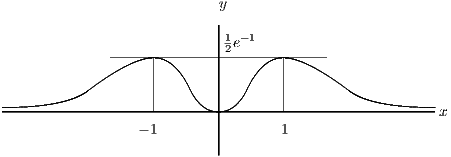
Since $y \to 0$ as $x \to \pm \infty$ , the sketch is:

PICT

For $C_{2}$ , the stationary points are again at $x = 0$ and $x = \pm 1$ . To classify the stationary points, we calculate the second derivative:

\frac{d^{2} y}{d x^{2}} = (1 - 3 x^{2} - 3 x^{3} + 3 x^{5}) e^{- x^{3}},

which is positive at $x = 0$ (a minimum) and negative at $x = 1$ (a maximum).

Since we cannot integrate this differential equation explicitly, we must compare $C_{2}$ with $C_{1}$ to see whether the value of $y$ at the maxima is indeed greater for $C_{2}$ than for $C_{1}$ .

For $0 < x < 1$ , $x^{3} < x^{2}$ , so $e^{x^{3}} < e^{x^{2}}$ and $e^{- x^{3}} > e^{- x^{2}}$ . Thus the gradient of $C_{2}$ is greater than the gradient of $C_{1}$ . Since both curves pass through the origin, we deduce that $C_{2}$ lies above $C_{1}$ for $0 < x \leq 1$ and therefore the maximum point $(1, k)$ on $C_{2}$ has $k > \frac{1}{2} e^{- 1}$ .

Post-mortem

You were probably surprised that the examiners didn’t ask you to sketch $C_{2}$ ; they usually do. It looks as if it could be done, because you know that $C_{2}$ passes through the origin and you can relate its slope, roughly at least, to that of $C_{1}$ , which you did sketch. The difficulty lies in determining its behaviour as $x \to \infty$ ; does $y \to 0$ as for $C_{1}$ ? In fact, it doesn’t; no reason why it should. Instead, $y \to 0.153 . . .$ . We shouldn’t have expected $C_{1}$ to asymptote to the $x$ -axis either; the fact that it does so is due to a rather delicate balancing of the two terms that determine its gradient.